In this document we detail the planned and additional analyses for our experiments. By default, all code elements are hidden and only the R output is visible. Individual code segments can be made visible through the respective buttons. To rerun complete analyses we recommend to download our zip file containg all analysis scripts.

Experiment 1

# Clean up memory
rm(list = ls())

# Experiment filenames
results_file <- "exp1/results"
crowflower_file <- "exp1/crowdflower_data"
invalid_answers_file <- "exp1/invalid_answers"
figure_path <- "plots/exp1-"

# Stimuli values (used to compute comprehension errors)
control <- 87  # % sick people without the drug
drug <- 47  # % sick people with the drug
# compute the true answer given the data
true_answer <- drug/control * 20

# Values reported by Tal and Wanksink to add to our plots as a comparison
bws_nochart <- 6.12
bws_chart <- 6.83
bws_p <- 0.04

Planned Analysis

library("plyr")
library("dplyr")

## 
## Attaching package: 'dplyr'

## The following objects are masked from 'package:plyr':
## 
##     arrange, count, desc, failwith, id, mutate, rename, summarise,
##     summarize

## The following objects are masked from 'package:stats':
## 
##     filter, lag

## The following objects are masked from 'package:base':
## 
##     intersect, setdiff, setequal, union

source("CI.helpers.R")

## Simple Bootstrap Routines (1.1-3 2008-04-30)

source("misc.helpers.R")
source("plotting functions.R")

## 
## Attaching package: 'gridExtra'

## The following object is masked from 'package:dplyr':
## 
##     combine

## 
## Attaching package: 'cowplot'

## The following object is masked from 'package:ggplot2':
## 
##     ggsave

# indicated whether we want ggplot to save the generated plots
save_plots <- FALSE
# print plots to screen
print_plots <- TRUE

Load data

# Load experiment data from csv file

if (exists("results_file")) {
    data <- read.csv(paste("data/", results_file, ".csv", sep = ""), sep = ",")
}

# Add crowdflower metadata (if exists)

if (exists("crowflower_file")) {
    crowdsourcedata <- read.csv(paste("data/", crowflower_file, ".csv", sep = ""), 
        sep = ",")
    data$code <- as.character(data$code)
    crowdsourcedata$completion_code <- as.character(crowdsourcedata$completion_code)
    data <- left_join(data, crowdsourcedata, by = c(code = "completion_code"))
    
    # Load country codes
    country_file <- "countries"
    countrydata <- read.csv(paste("data/", country_file, ".csv", sep = ""), 
        sep = ",")
}

# Add mturk metadata (if exists)

if (exists("mturk_file")) {
    crowdsourcedata <- read.csv(paste("data/", mturk_file, ".csv", sep = ""), 
        sep = ",")
    data$code <- as.character(data$code)
    crowdsourcedata$Answer.completion_code <- as.character(crowdsourcedata$Answer.completion_code)
    data <- left_join(data, crowdsourcedata, by = c(code = "Answer.completion_code"))
}

Invalid jobs

# Utility function for printing percentages
percent <- function(x, n) {
    if (x/n < 0.01) 
        r <- 1 else r <- 0
    paste(" (", format_number(100 * x/n, r), "%)", sep = "")
}

print.title("Invalid jobs")

## 
## ###################################
## # Invalid jobs 
## ###################################

data_invalid <- read.csv(paste("data/", invalid_answers_file, ".csv", sep = ""), 
    sep = ",")
n_valid <- nrow(data)
n_invalid <- nrow(data_invalid)
n <- n_valid + n_invalid
cat("Valid jobs:   ", n_valid, "\n")

## Valid jobs:    123

cat("Invalid jobs: ", n_invalid, "\n\n")

## Invalid jobs:  25

# 
n_failed_attention <- nrow(data_invalid[data_invalid$test_question != "common_cold", 
    ])
n_abnormal_time <- nrow(data_invalid[data_invalid$time_taken < 30 | data_invalid$time_taken > 
    15 * 60, ])
n_previous_study <- nrow(data_invalid[data_invalid$previous_study == "yes", 
    ])
cat("Failed attention check:   ", n_failed_attention, percent(n_failed_attention, 
    n), "\n", sep = "")

## Failed attention check:   7 (5%)

cat("Abnormal completion time: ", n_abnormal_time, percent(n_abnormal_time, 
    n), "\n", sep = "")

## Abnormal completion time: 4 (3%)

cat("Did study before:         ", n_previous_study, percent(n_previous_study, 
    n), "\n", sep = "")

## Did study before:         18 (10%)

Sample size, completion time and demographics

# Sample size

N <- nrow(data)
cat("Total sample size:  ", N, "\n")

## Total sample size:   123

cat("n =", sum(data$condition == "no_graph"), "for the no-chart condition\n")

## n = 62 for the no-chart condition

cat("n =", sum(data$condition == "graph"), "for the chart condition\n\n")

## n = 61 for the chart condition

# Job completion time

mt <- median(data$time_taken)
cat("Median job completion time:", format_number(mt/60, 2), "minutes.\n\n")

## Median job completion time: 2.4 minutes.

# Countries

if (exists("crowflower_file")) {
    data$country <- sapply(data$X_country, function(code) countrydata$name[match(code, 
        countrydata$alpha.3)])
    data$subregion <- sapply(data$X_country, function(code) countrydata$sub.region[match(code, 
        countrydata$alpha.3)])
    data$continent <- sapply(data$X_country, function(code) countrydata$region[match(code, 
        countrydata$alpha.3)])
    cat("Number of different countries:", length(unique(data$country)), "\n")
    print.percents(data$continent)
}

## Number of different countries: 32 
##             n  %
## 1   Europe 68 55
## 2 Americas 34 28
## 3     Asia 21 17

# Gender distribution

# Column is present in all but experiment 3
if ("gender" %in% colnames(data)) {
    cat("\nGender:\n")
    print.percents(data$gender)
}

## 
## Gender:
##           n  %
## 1   male 80 65
## 2 female 43 35

# Age

# Column is present in all but experiment 3
if ("age" %in% colnames(data)) {
    cat("\nMean age:", round(mean(data$age)), "\n")
}

## 
## Mean age: 35

# Education

# Column is present in all but experiment 3
if ("education" %in% colnames(data)) {
    cat("\nEducation:\n")
    print.percents(data$education)
}

## 
## Education:
##                    n  %
## 1 college_or_more 59 48
## 2    some_college 34 28
## 3     high-school 27 22
## 4         neither  3  2

Analysis of dependent variables

##### Retrieve data

# Extract judgments of drug efficacy (values between 1 and 9).  Experiment 1
# and experiments 2-4 use different question wordings, hence we look at two
# possible columns.

# Column is present in experiment 1, which replicates the question from BwS
# experiment 1
if ("effectiveness" %in% colnames(data)) {
    eff_nograph <- data[data$condition == "no_graph", ]$effectiveness
    eff_graph <- data[data$condition == "graph", ]$effectiveness
    variable_name <- "Perceived effectiveness"
}

# Column is present in experiments 2-4, which replicate the question from
# BwS experiment 2
if ("believe_in_effectiveness" %in% colnames(data)) {
    eff_nograph <- data[data$condition == "no_graph", ]$believe_in_effectiveness
    eff_graph <- data[data$condition == "graph", ]$believe_in_effectiveness
    variable_name <- "Belief in efficacy"
}

# Extract belief in drug from the second question (yes = not effective, no =
# effective).

# Column is present in experiment 1 only.
if ("reduces_sickness" %in% colnames(data)) {
    yesno_to_01 <- function(x) {
        if (x == "yes") 
            1 else if (x == "no") 
            0 else NA
    }
    ill_nograph <- data[data$condition == "no_graph", ]$reduces_sickness
    ill_graph <- data[data$condition == "graph", ]$reduces_sickness
    ill_nograph <- sapply(ill_nograph, yesno_to_01)
    ill_graph <- sapply(ill_graph, yesno_to_01)
}

# Extract answers to comprehension question

num_nograph <- data[data$condition == "no_graph", ]$comprehension
num_graph <- data[data$condition == "graph", ]$comprehension

##### Descriptive and inferential statistics

Judgment of efficacy

##### CIs for judgment of efficacy on a 1--9 scale

mean_eff_nograph <- meanCI.bootstrap(eff_nograph)
mean_eff_graph <- meanCI.bootstrap(eff_graph)
mean_eff_diff <- diffMeanCI.bootstrap(eff_graph, eff_nograph)

print.title(variable_name)

## 
## ###################################
## # Perceived effectiveness 
## ###################################

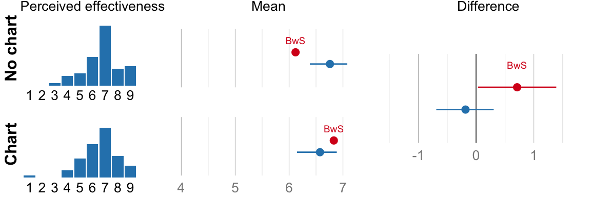
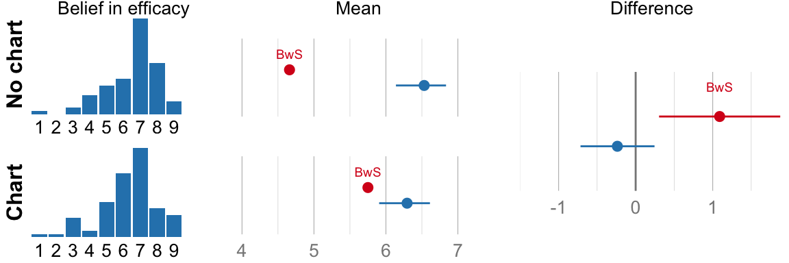
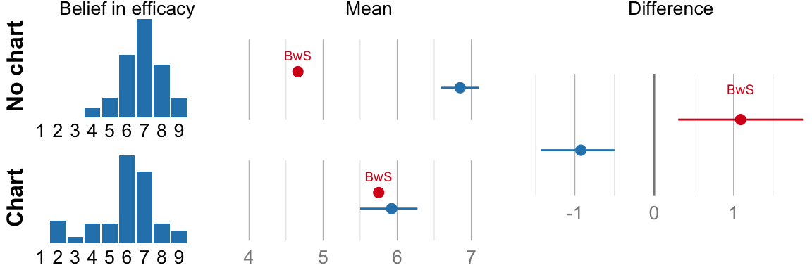
cat("Mean efficacy no-chart: ", format_ci(mean_eff_nograph), "\n")

## Mean efficacy no-chart:  6.8, CI [6.4, 7.1]

cat("Mean efficacy chart:    ", format_ci(mean_eff_graph), "\n")

## Mean efficacy chart:     6.6, CI [6.1, 6.9]

cat("Difference:             ", format_ci(mean_eff_diff), "\n")

## Difference:              -0.18, CI [-0.69, 0.30]

# NHST version for comparison (used in the original paper, but not part of
# this planned analysis)

ttest <- t.test(eff_graph, eff_nograph)
mean_eff_diff_normal <- c(mean(eff_graph) - mean(eff_nograph), ttest$conf.int[1], 
    ttest$conf.int[2])
cat("(using a t-test)        ", format_ci(mean_eff_diff_normal), "p =", format_number(ttest$p.value), 
    "\n")

## (using a t-test)         -0.18, CI [-0.69, 0.33] p = 0.48

# Display distributions of efficacy judgments and confidence intervals for
# estimates

## compile CIs and BwS results into a dataframe for plotting
eff_df <- NULL
eff_df <- add.ci.to.df(mean_eff_nograph, "no chart", "ours", eff_df)
eff_df <- add.ci.to.df(c(bws_nochart, bws_nochart, bws_nochart), "no chart", 
    "BwS", eff_df)
eff_df <- add.ci.to.df(mean_eff_graph, "chart", "ours", eff_df)
eff_df <- add.ci.to.df(c(bws_chart, bws_chart, bws_chart), "chart", "BwS", eff_df)

eff_diff_df <- NULL
eff_diff_df <- add.ci.to.df(mean_eff_diff, " ", "ours")
eff_diff_df <- add.ci.to.df(ci_from_p(bws_chart - bws_nochart, bws_p), " ", 
    "BwS", eff_diff_df)

if (variable_name == "Belief in efficacy") {
    # plotting for experiments 2-4
    eff.hist.no_chart <- histo(eff_nograph, 9, "no chart", 0, 1)
    eff.hist.chart <- histo(eff_graph, 9, "chart", 0, 1)
    
    eff.cis <- perceived.effectiveness.ciplot(eff_df, eff_diff_df)
    
    plot <- drawVertical(eff.hist.no_chart, eff.hist.chart, eff.cis, name.eff.exp24, 
        "Difference")
    if (save_plots) 
        save_plot(paste(sep = "", figure_path, "believe_in_efficacy_plot.pdf"), 
            plot, base_aspect_ratio = 3, base_height = 2)
    if (print_plots) 
        print(plot)
    
} else {
    # plotting for experiment 1
    eff.hist.no_chart <- histo(eff_nograph, 9, "no chart", 0, 1)
    eff.hist.chart <- histo(eff_graph, 9, "chart", 0, 1)
    eff.cis <- perceived.effectiveness.1.ciplot(eff_df, eff_diff_df)
    
    plot <- drawVertical(eff.hist.no_chart, eff.hist.chart, eff.cis, name.eff.exp1, 
        "Difference")
    if (save_plots) 
        save_plot(paste(sep = "", figure_path, "perceived_effectiveness_plot.pdf"), 
            plot, base_aspect_ratio = 3, base_height = 2)
    if (print_plots) 
        print(plot)
}

Binary belief in efficacy

##### CIs for binary belief in efficacy

# Column is present in experiment 1 only, as subsequent experiments didn't
# include that question.
if ("reduces_sickness" %in% colnames(data)) {
    
    mean_ill_nograph <- propCI(sum(ill_nograph == 1), length(ill_nograph))
    mean_ill_graph <- propCI(sum(ill_graph == 1), length(ill_graph))
    mean_ill_diff <- diffpropCI(sum(ill_graph == 1), length(ill_graph), sum(ill_nograph == 
        1), length(ill_nograph))
    
    print.title("Belief in efficacy (binary)")
    cat("Proportion of 'yes' no-chart: ", format_ci(mean_ill_nograph, percent = TRUE), 
        "\n")
    cat("Proportion of 'yes' chart:    ", format_ci(mean_ill_graph, percent = TRUE), 
        "\n")
    cat("Difference:                   ", format_ci(mean_ill_diff, percent = TRUE), 
        "\n")
    
    # NHST version for comparison (used in the original paper, but not part of
    # this planned analysis)
    
    yes <- c(sum(ill_graph == 1), sum(ill_nograph == 1))
    all <- c(length(ill_graph), length(ill_nograph))
    proptest <- prop.test(yes, all, correct = F)  # disable continuity correction to get the same p-value
    mean_ill_diff_2 <- c(yes[1]/all[1] - yes[2]/all[2], proptest$conf.int[1], 
        proptest$conf.int[2])
    cat("(using an X-squared test)     ", format_ci(mean_ill_diff_2, percent = TRUE), 
        "p =", format_number(proptest$p.value), "\n")
    
    # Plot our results in comparison to the BwS results
    
    # Tal and Wanksink's results
    bws.cis.no_graph <- propCI(21, 31)
    bws.cis.graph <- propCI(28, 29)
    bws.cis.diff <- diffpropCI(28, 29, 21, 31)
    
    # construct the dataframes for plotting
    efficiency.df <- NULL
    efficiency.df <- add.ci.to.df(mean_ill_nograph, "no chart", "ours", efficiency.df)
    efficiency.df <- add.ci.to.df(mean_ill_graph, "chart", "ours", efficiency.df)
    efficiency.df <- add.ci.to.df(bws.cis.no_graph, "no chart", "BwS", efficiency.df)
    efficiency.df <- add.ci.to.df(bws.cis.graph, "chart", "BwS", efficiency.df)
    
    efficiency.diff.df <- NULL
    efficiency.diff.df <- add.ci.to.df(mean_ill_diff, " ", "ours", efficiency.diff.df)
    efficiency.diff.df <- add.ci.to.df(bws.cis.diff, " ", "BwS", efficiency.diff.df)
    
    # plot
    efficiency.ciplot <- efficacy.belief.ciplot(efficiency.df, efficiency.diff.df)
    efficiency.plot <- drawHorizontalEfficiency(efficiency.ciplot, "Belief in efficacy", 
        "Difference")
    if (save_plots) 
        save_plot(paste(sep = "", figure_path, "belief_in_efficacy_plot.pdf"), 
            efficiency.plot, base_aspect_ratio = 4, base_height = 1.5)
    if (print_plots) 
        print(efficiency.plot)
}

## 
## ###################################
## # Belief in efficacy (binary) 
## ###################################
## 
## Proportion of 'yes' no-chart:  90%, CI [80%, 95%] 
## Proportion of 'yes' chart:     87%, CI [76%, 93%] 
## Difference:                    -3.4%, CI [-16%, 8.4%] 
## (using an X-squared test)      -3.4%, CI [-15%, 7.8%] p = 0.55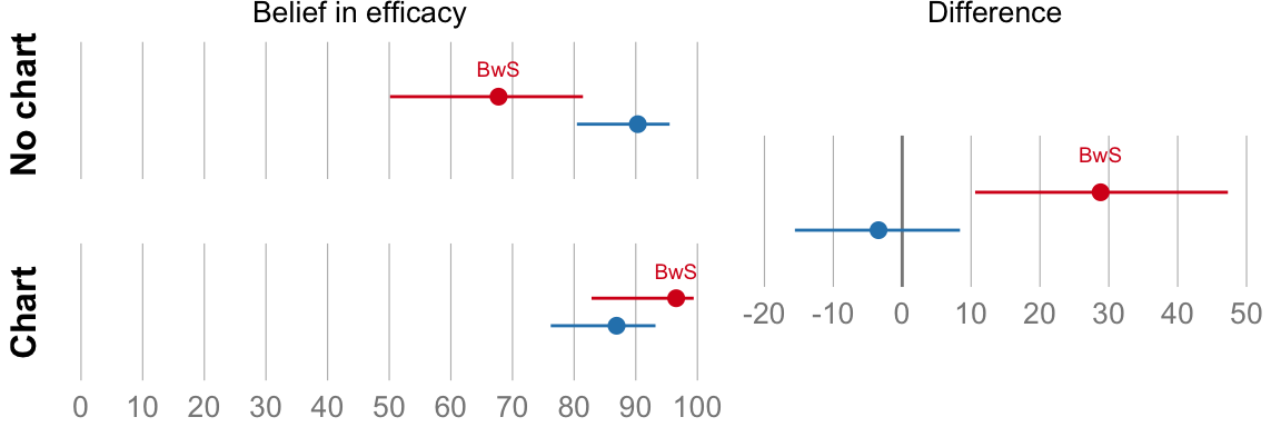

Comprehension question

#### CIs for errors at the comprehension question

# Define error
psick <- drug/control
logodds <- function(p) {
    log(p/(1 - p))
}
logodds.psick <- logodds(psick)
error <- function(n) {
    n[n == 0] <- 0.1
    n[n == 20] <- 19.9
    abs(logodds(n/20) - logodds.psick)
}

# Compute errors
data$error <- error(data$comprehension)
err_nograph <- error(num_nograph)
err_graph <- error(num_graph)

# Use geometric mean to reduce the influence of outliers and increase the
# weight of close-to-exact answers
mean_err_nograph <- geomMeanCI.bootstrap(err_nograph)
mean_err_graph <- geomMeanCI.bootstrap(err_graph)
mean_err_diff <- ratioGeomMeanCI.bootstrap(err_graph, err_nograph)
print.title("Comprehension error")

## 
## ###################################
## # Comprehension error 
## ###################################

cat("Geometric mean error no-chart: ", format_ci(mean_err_nograph), "\n")

## Geometric mean error no-chart:  0.66, CI [0.49, 0.88]

cat("Geometric mean error chart:    ", format_ci(mean_err_graph), "\n")

## Geometric mean error chart:     0.43, CI [0.33, 0.56]

cat("Ratio:                         ", format_ci(mean_err_diff), "\n")

## Ratio:                          0.65, CI [0.44, 0.98]

# Plot raw responses and confidence intervals

comp.hist.no_chart <- histo(num_nograph, 20, "no chart", true_answer, 1)
comp.hist.chart <- histo(num_graph, 20, "chart", true_answer, 1)

# construct the dataframes for plotting
comprehension.df <- NULL
comprehension.df <- add.ci.to.df(mean_err_nograph, "no chart", "ours", comprehension.df)
comprehension.df <- add.ci.to.df(mean_err_graph, "chart", "ours", comprehension.df)

comprehension.diff.df <- NULL
comprehension.diff.df <- add.ci.to.df(mean_err_diff, " ", "ours", comprehension.diff.df)

# plot
comp.cis <- comprehension.ciplot(comprehension.df, comprehension.diff.df)
comp.plot <- drawVerticalComp(comp.hist.no_chart, comp.hist.chart, comp.cis, 
    "Comprehension error", "Error ratio")
if (save_plots) save_plot(paste(sep = "", figure_path, "comprehension_plot.pdf"), 
    comp.plot, base_aspect_ratio = 3, base_height = 2)
if (print_plots) print(comp.plot)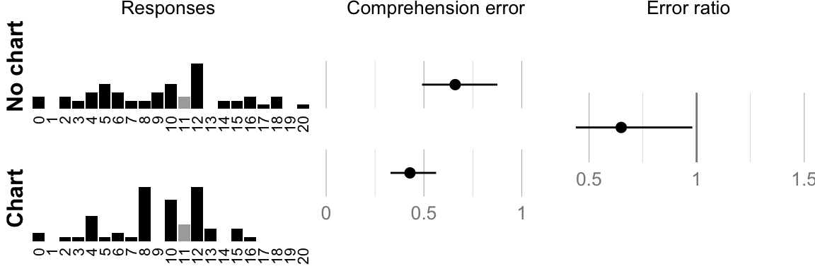

Additional Analysis

Bias in responses

cat("Mean response no-chart: ", format_ci(meanCI.bootstrap(num_nograph), sigdigits = 3), 
    "\n")

## Mean response no-chart:  9.19, CI [7.91, 10.4]

cat("Mean response chart:    ", format_ci(meanCI.bootstrap(num_graph), sigdigits = 3), 
    "\n")

## Mean response chart:     9.13, CI [8.14, 9.97]

cat("Mean difference:        ", format_ci(diffMeanCI.bootstrap(num_graph, num_nograph)), 
    "\n")

## Mean difference:         -0.062, CI [-1.67, 1.40]

# Justifications from those who responded 'no' to the belief question. This
# data was not reported, but it informed the design of our polarization
# question (see section 6.1)

Justifications to ‘no’ answers

whyno <- as.character(data$why_answered_no)
whyno <- whyno[whyno != ""]
cat(whyno, sep = "\n-> ")

## this is how i think
## -> it depend on human body and immune system
## -> because more side effect of medication
## -> Not all people react the same to the medication. It takes a lot of time to demonstrate the usefulness of the medication.
## -> I do not belive that the medications can actually increase immunity. Drugs act on the symptoms.
## -> the drug busts the immune system. There is no way to know if this is the case nor if the user would get sick without it.
## -> i dont belive in miraculous drugs if they found it the studies where over by now
## -> I didn't compute it in the way that the follow up question did, which assumed that those 20 people would by default all get sick. I thought this lower sickness rate could simply be due to extraneous factors. And since the remaining percentage of people getting ill was still rather high, I chose NO here.
## -> It boost immune system still the illnes remains
## -> I simply don't believe in such medication, never had any proof.
## -> The medication does not reduce the disease
## -> The drug is implicitly stated as boosting the human immune system, not fight infections.
## -> Because you can't cure cold.
## -> Because it increases immunity, but does not cure disease

Experiment 2

# Clean up memory
rm(list = ls())

# Experiment filenames
results_file <- "exp2/results"
crowflower_file <- "exp2/crowdflower_data"
invalid_answers_file <- "exp2/invalid_answers"
figure_path <- "plots/exp2-"

# Stimuli values (used to compute comprehension errors)
control <- 83  # % sick people without the drug
drug <- 63  # % sick people with the drug
# compute the true answer given the data
true_answer <- 63/83 * 20

# Values reported by Tal and Wanksink to add to our plots as a comparison
bws_nochart <- 4.66
bws_chart <- 5.75
bws_p <- 0.0066

Planned Analysis

library("plyr")
library("dplyr")

source("CI.helpers.R")
source("misc.helpers.R")
source("plotting functions.R")

# indicated whether we want ggplot to save the generated plots
save_plots <- FALSE
# print plots to screen
print_plots <- TRUE

Load data

# Load experiment data from csv file

if (exists("results_file")) {
    data <- read.csv(paste("data/", results_file, ".csv", sep = ""), sep = ",")
}

# Add crowdflower metadata (if exists)

if (exists("crowflower_file")) {
    crowdsourcedata <- read.csv(paste("data/", crowflower_file, ".csv", sep = ""), 
        sep = ",")
    data$code <- as.character(data$code)
    crowdsourcedata$completion_code <- as.character(crowdsourcedata$completion_code)
    data <- left_join(data, crowdsourcedata, by = c(code = "completion_code"))
    
    # Load country codes
    country_file <- "countries"
    countrydata <- read.csv(paste("data/", country_file, ".csv", sep = ""), 
        sep = ",")
}

# Add mturk metadata (if exists)

if (exists("mturk_file")) {
    crowdsourcedata <- read.csv(paste("data/", mturk_file, ".csv", sep = ""), 
        sep = ",")
    data$code <- as.character(data$code)
    crowdsourcedata$Answer.completion_code <- as.character(crowdsourcedata$Answer.completion_code)
    data <- left_join(data, crowdsourcedata, by = c(code = "Answer.completion_code"))
}

Invalid Jobs

# Utility function for printing percentages
percent <- function(x, n) {
    if (x/n < 0.01) 
        r <- 1 else r <- 0
    paste(" (", format_number(100 * x/n, r), "%)", sep = "")
}

data_invalid <- read.csv(paste("data/", invalid_answers_file, ".csv", sep = ""), 
    sep = ",")
n_valid <- nrow(data)
n_invalid <- nrow(data_invalid)
n <- n_valid + n_invalid
cat("Valid jobs:   ", n_valid, "\n")

## Valid jobs:    164

cat("Invalid jobs: ", n_invalid, "\n\n")

## Invalid jobs:  32

# 
n_failed_attention <- nrow(data_invalid[data_invalid$test_question != "common_cold", 
    ])
n_abnormal_time <- nrow(data_invalid[data_invalid$time_taken < 30 | data_invalid$time_taken > 
    15 * 60, ])
n_previous_study <- nrow(data_invalid[data_invalid$previous_study == "yes", 
    ])
cat("Failed attention check:   ", n_failed_attention, percent(n_failed_attention, 
    n), "\n", sep = "")

## Failed attention check:   6 (3%)

cat("Abnormal completion time: ", n_abnormal_time, percent(n_abnormal_time, 
    n), "\n", sep = "")

## Abnormal completion time: 3 (2%)

cat("Did study before:         ", n_previous_study, percent(n_previous_study, 
    n), "\n", sep = "")

## Did study before:         20 (10%)

Sample size, completion time and demographics

# Sample size

N <- nrow(data)
cat("Total sample size:  ", N, "\n")

## Total sample size:   164

cat("n =", sum(data$condition == "no_graph"), "for the no-chart condition\n")

## n = 79 for the no-chart condition

cat("n =", sum(data$condition == "graph"), "for the chart condition\n\n")

## n = 85 for the chart condition

# Job completion time

mt <- median(data$time_taken)
cat("Median job completion time:", format_number(mt/60, 2), "minutes.\n\n")

## Median job completion time: 2.0 minutes.

# Countries

if (exists("crowflower_file")) {
    data$country <- sapply(data$X_country, function(code) countrydata$name[match(code, 
        countrydata$alpha.3)])
    data$subregion <- sapply(data$X_country, function(code) countrydata$sub.region[match(code, 
        countrydata$alpha.3)])
    data$continent <- sapply(data$X_country, function(code) countrydata$region[match(code, 
        countrydata$alpha.3)])
    cat("Number of different countries:", length(unique(data$country)), "\n")
    print.percents(data$continent)
}

## Number of different countries: 34 
##             n  %
## 1   Europe 91 55
## 2 Americas 37 23
## 3     Asia 32 20
## 4   Africa  2  1
## 5  Oceania  2  1

# Gender distribution

# Column is present in all but experiment 3
if ("gender" %in% colnames(data)) {
    cat("\nGender:\n")
    print.percents(data$gender)
}

## 
## Gender:
##            n  %
## 1   male 118 72
## 2 female  46 28

# Age

# Column is present in all but experiment 3
if ("age" %in% colnames(data)) {
    cat("\nMean age:", round(mean(data$age)), "\n")
}

## 
## Mean age: 34

# Education

# Column is present in all but experiment 3
if ("education" %in% colnames(data)) {
    cat("\nEducation:\n")
    print.percents(data$education)
}

## 
## Education:
##                    n  %
## 1 college_or_more 94 57
## 2    some_college 44 27
## 3     high-school 22 13
## 4         neither  4  2

Analysis of dependent variables

##### Retrieve data

# Extract judgments of drug efficacy (values between 1 and 9).  Experiment 1
# and experiments 2-4 use different question wordings, hence we look at two
# possible columns.

# Column is present in experiment 1, which replicates the question from BwS
# experiment 1
if ("effectiveness" %in% colnames(data)) {
    eff_nograph <- data[data$condition == "no_graph", ]$effectiveness
    eff_graph <- data[data$condition == "graph", ]$effectiveness
    variable_name <- "Perceived effectiveness"
}

# Column is present in experiments 2-4, which replicate the question from
# BwS experiment 2
if ("believe_in_effectiveness" %in% colnames(data)) {
    eff_nograph <- data[data$condition == "no_graph", ]$believe_in_effectiveness
    eff_graph <- data[data$condition == "graph", ]$believe_in_effectiveness
    variable_name <- "Belief in efficacy"
}

# Extract belief in drug from the second question (yes = not effective, no =
# effective).

# Column is present in experiment 1 only.
if ("reduces_sickness" %in% colnames(data)) {
    yesno_to_01 <- function(x) {
        if (x == "yes") 
            1 else if (x == "no") 
            0 else NA
    }
    ill_nograph <- data[data$condition == "no_graph", ]$reduces_sickness
    ill_graph <- data[data$condition == "graph", ]$reduces_sickness
    ill_nograph <- sapply(ill_nograph, yesno_to_01)
    ill_graph <- sapply(ill_graph, yesno_to_01)
}

# Extract answers to comprehension question

num_nograph <- data[data$condition == "no_graph", ]$comprehension
num_graph <- data[data$condition == "graph", ]$comprehension

Belief in efficacy

##### CIs for judgment of efficacy on a 1--9 scale

mean_eff_nograph <- meanCI.bootstrap(eff_nograph)
mean_eff_graph <- meanCI.bootstrap(eff_graph)
mean_eff_diff <- diffMeanCI.bootstrap(eff_graph, eff_nograph)

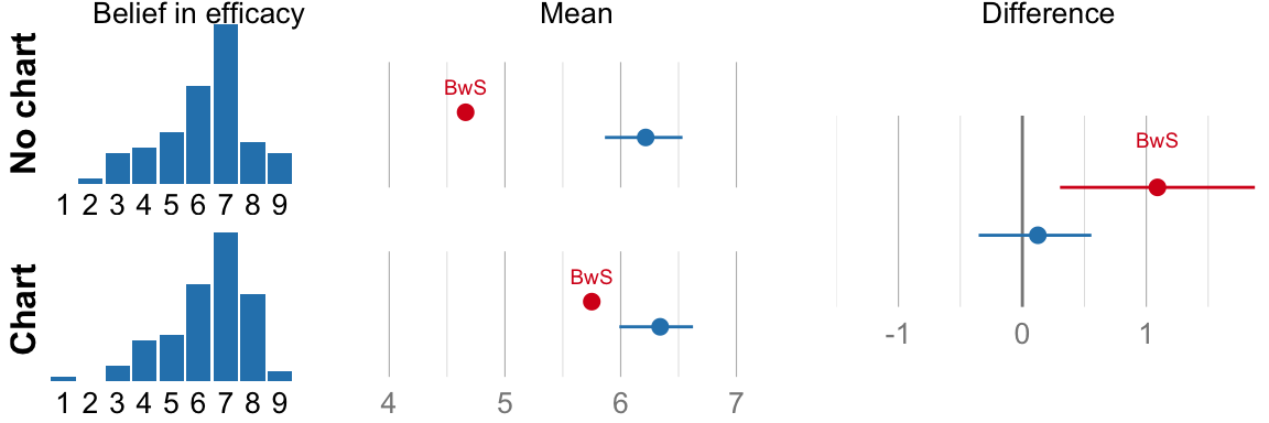
cat("Mean efficacy no-chart: ", format_ci(mean_eff_nograph), "\n")

## Mean efficacy no-chart:  6.5, CI [6.1, 6.8]

cat("Mean efficacy chart:    ", format_ci(mean_eff_graph), "\n")

## Mean efficacy chart:     6.3, CI [5.9, 6.6]

cat("Difference:             ", format_ci(mean_eff_diff), "\n")

## Difference:              -0.24, CI [-0.72, 0.24]

# NHST version for comparison (used in the original paper, but not part of
# this planned analysis)

ttest <- t.test(eff_graph, eff_nograph)
mean_eff_diff_normal <- c(mean(eff_graph) - mean(eff_nograph), ttest$conf.int[1], 
    ttest$conf.int[2])
cat("(using a t-test)        ", format_ci(mean_eff_diff_normal), "p =", format_number(ttest$p.value), 
    "\n")

## (using a t-test)         -0.24, CI [-0.73, 0.26] p = 0.34

# Display distributions of efficacy judgments and confidence intervals for
# estimates

## compile CIs and BwS results into a dataframe for plotting
eff_df <- NULL
eff_df <- add.ci.to.df(mean_eff_nograph, "no chart", "ours", eff_df)
eff_df <- add.ci.to.df(c(bws_nochart, bws_nochart, bws_nochart), "no chart", 
    "BwS", eff_df)
eff_df <- add.ci.to.df(mean_eff_graph, "chart", "ours", eff_df)
eff_df <- add.ci.to.df(c(bws_chart, bws_chart, bws_chart), "chart", "BwS", eff_df)

eff_diff_df <- NULL
eff_diff_df <- add.ci.to.df(mean_eff_diff, " ", "ours")
eff_diff_df <- add.ci.to.df(ci_from_p(bws_chart - bws_nochart, bws_p), " ", 
    "BwS", eff_diff_df)

if (variable_name == "Belief in efficacy") {
    # plotting for experiments 2-4
    eff.hist.no_chart <- histo(eff_nograph, 9, "no chart", 0, 1)
    eff.hist.chart <- histo(eff_graph, 9, "chart", 0, 1)
    
    eff.cis <- perceived.effectiveness.ciplot(eff_df, eff_diff_df)
    
    plot <- drawVertical(eff.hist.no_chart, eff.hist.chart, eff.cis, name.eff.exp24, 
        "Difference")
    if (save_plots) 
        save_plot(paste(sep = "", figure_path, "believe_in_efficacy_plot.pdf"), 
            plot, base_aspect_ratio = 3, base_height = 2)
    if (print_plots) 
        print(plot)
    
} else {
    # plotting for experiment 1
    eff.hist.no_chart <- histo(eff_nograph, 9, "no chart", 0, 1)
    eff.hist.chart <- histo(eff_graph, 9, "chart", 0, 1)
    eff.cis <- perceived.effectiveness.1.ciplot(eff_df, eff_diff_df)
    
    plot <- drawVertical(eff.hist.no_chart, eff.hist.chart, eff.cis, name.eff.exp1, 
        "Difference")
    if (save_plots) 
        save_plot(paste(sep = "", figure_path, "perceived_effectiveness_plot.pdf"), 
            plot, base_aspect_ratio = 3, base_height = 2)
    if (print_plots) 
        print(plot)
}

##### CIs for binary belief in efficacy

# Column is present in experiment 1 only, as subsequent experiments didn't
# include that question.
if ("reduces_sickness" %in% colnames(data)) {
    
    mean_ill_nograph <- propCI(sum(ill_nograph == 1), length(ill_nograph))
    mean_ill_graph <- propCI(sum(ill_graph == 1), length(ill_graph))
    mean_ill_diff <- diffpropCI(sum(ill_graph == 1), length(ill_graph), sum(ill_nograph == 
        1), length(ill_nograph))
    
    print.title("Belief in efficacy (binary)")
    cat("Proportion of 'yes' no-chart: ", format_ci(mean_ill_nograph, percent = TRUE), 
        "\n")
    cat("Proportion of 'yes' chart:    ", format_ci(mean_ill_graph, percent = TRUE), 
        "\n")
    cat("Difference:                   ", format_ci(mean_ill_diff, percent = TRUE), 
        "\n")
    
    # NHST version for comparison (used in the original paper, but not part of
    # this planned analysis)
    
    yes <- c(sum(ill_graph == 1), sum(ill_nograph == 1))
    all <- c(length(ill_graph), length(ill_nograph))
    proptest <- prop.test(yes, all, correct = F)  # disable continuity correction to get the same p-value
    mean_ill_diff_2 <- c(yes[1]/all[1] - yes[2]/all[2], proptest$conf.int[1], 
        proptest$conf.int[2])
    cat("(using an X-squared test)     ", format_ci(mean_ill_diff_2, percent = TRUE), 
        "p =", format_number(proptest$p.value), "\n")
    
    # Plot our results in comparison to the BwS results
    
    # Tal and Wanksink's results
    bws.cis.no_graph <- propCI(21, 31)
    bws.cis.graph <- propCI(28, 29)
    bws.cis.diff <- diffpropCI(28, 29, 21, 31)
    
    # construct the dataframes for plotting
    efficiency.df <- NULL
    efficiency.df <- add.ci.to.df(mean_ill_nograph, "no chart", "ours", efficiency.df)
    efficiency.df <- add.ci.to.df(mean_ill_graph, "chart", "ours", efficiency.df)
    efficiency.df <- add.ci.to.df(bws.cis.no_graph, "no chart", "BwS", efficiency.df)
    efficiency.df <- add.ci.to.df(bws.cis.graph, "chart", "BwS", efficiency.df)
    
    efficiency.diff.df <- NULL
    efficiency.diff.df <- add.ci.to.df(mean_ill_diff, " ", "ours", efficiency.diff.df)
    efficiency.diff.df <- add.ci.to.df(bws.cis.diff, " ", "BwS", efficiency.diff.df)
    
    # plot
    efficiency.ciplot <- efficacy.belief.ciplot(efficiency.df, efficiency.diff.df)
    efficiency.plot <- drawHorizontalEfficiency(efficiency.ciplot, "Belief in efficacy", 
        "Difference")
    if (save_plots) 
        save_plot(paste(sep = "", figure_path, "belief_in_efficacy_plot.pdf"), 
            efficiency.plot, base_aspect_ratio = 4, base_height = 1.5)
    if (print_plots) 
        print(efficiency.plot)
}

Comprehension question

#### CIs for errors at the comprehension question

# Define error
psick <- drug/control
logodds <- function(p) {
    log(p/(1 - p))
}
logodds.psick <- logodds(psick)
error <- function(n) {
    n[n == 0] <- 0.1
    n[n == 20] <- 19.9
    abs(logodds(n/20) - logodds.psick)
}

# Compute errors
data$error <- error(data$comprehension)
err_nograph <- error(num_nograph)
err_graph <- error(num_graph)

# Use geometric mean to reduce the influence of outliers and increase the
# weight of close-to-exact answers
mean_err_nograph <- geomMeanCI.bootstrap(err_nograph)
mean_err_graph <- geomMeanCI.bootstrap(err_graph)
mean_err_diff <- ratioGeomMeanCI.bootstrap(err_graph, err_nograph)
print.title("Comprehension error")

## 
## ###################################
## # Comprehension error 
## ###################################

cat("Geometric mean error no-chart: ", format_ci(mean_err_nograph), "\n")

## Geometric mean error no-chart:  0.83, CI [0.62, 1.06]

cat("Geometric mean error chart:    ", format_ci(mean_err_graph), "\n")

## Geometric mean error chart:     0.75, CI [0.56, 0.97]

cat("Ratio:                         ", format_ci(mean_err_diff), "\n")

## Ratio:                          0.91, CI [0.63, 1.35]

# Plot raw responses and confidence intervals

comp.hist.no_chart <- histo(num_nograph, 20, "no chart", true_answer, 1)
comp.hist.chart <- histo(num_graph, 20, "chart", true_answer, 1)

# construct the dataframes for plotting
comprehension.df <- NULL
comprehension.df <- add.ci.to.df(mean_err_nograph, "no chart", "ours", comprehension.df)
comprehension.df <- add.ci.to.df(mean_err_graph, "chart", "ours", comprehension.df)

comprehension.diff.df <- NULL
comprehension.diff.df <- add.ci.to.df(mean_err_diff, " ", "ours", comprehension.diff.df)

# plot
comp.cis <- comprehension.ciplot(comprehension.df, comprehension.diff.df)
comp.plot <- drawVerticalComp(comp.hist.no_chart, comp.hist.chart, comp.cis, 
    "Comprehension error", "Error ratio")
if (save_plots) save_plot(paste(sep = "", figure_path, "comprehension_plot.pdf"), 
    comp.plot, base_aspect_ratio = 3, base_height = 2)
if (print_plots) print(comp.plot)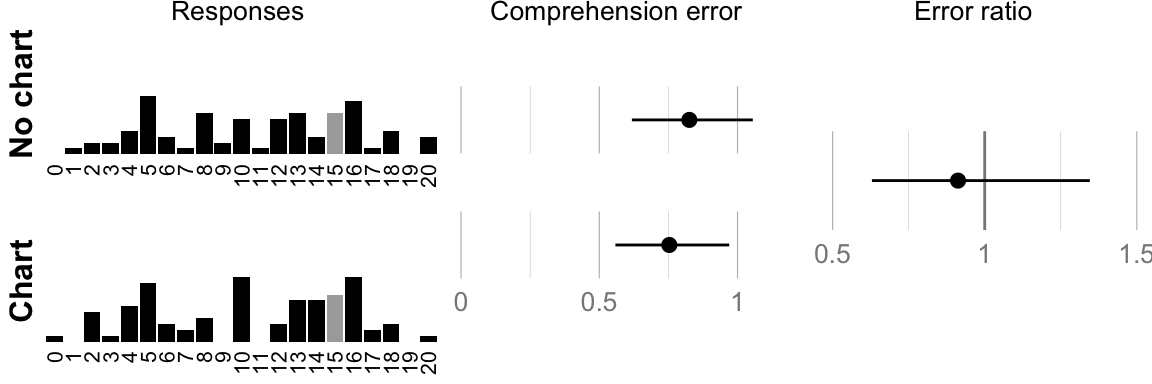

Experiment 3

# Clean up memory
rm(list = ls())

# Experiment filenames
results_file <- "exp3/results"
crowflower_file <- "exp3/crowdflower_data"
invalid_answers_file <- "exp3/invalid_answers"
figure_path <- "plots/exp3-"

# Stimuli values (used to compute comprehension errors)
control <- 83  # % sick people without the drug
drug <- 63  # % sick people with the drug
# compute the true answer given the data
true_answer <- 63/83 * 20

# Values reported by Tal and Wanksink to add to our plots as a comparison
bws_nochart <- 4.66
bws_chart <- 5.75
bws_p <- 0.0066

Planned Analysis

library("plyr")
library("dplyr")

source("CI.helpers.R")
source("misc.helpers.R")
source("plotting functions.R")

# indicated whether we want ggplot to save the generated plots
save_plots <- FALSE
# print plots to screen
print_plots <- TRUE

Load data

# Load experiment data from csv file

if (exists("results_file")) {
    data <- read.csv(paste("data/", results_file, ".csv", sep = ""), sep = ",")
}

# Add crowdflower metadata (if exists)

if (exists("crowflower_file")) {
    crowdsourcedata <- read.csv(paste("data/", crowflower_file, ".csv", sep = ""), 
        sep = ",")
    data$code <- as.character(data$code)
    crowdsourcedata$completion_code <- as.character(crowdsourcedata$completion_code)
    data <- left_join(data, crowdsourcedata, by = c(code = "completion_code"))
    
    # Load country codes
    country_file <- "countries"
    countrydata <- read.csv(paste("data/", country_file, ".csv", sep = ""), 
        sep = ",")
}

# Add mturk metadata (if exists)

if (exists("mturk_file")) {
    crowdsourcedata <- read.csv(paste("data/", mturk_file, ".csv", sep = ""), 
        sep = ",")
    data$code <- as.character(data$code)
    crowdsourcedata$Answer.completion_code <- as.character(crowdsourcedata$Answer.completion_code)
    data <- left_join(data, crowdsourcedata, by = c(code = "Answer.completion_code"))
}

Invalid jobs

# Utility function for printing percentages
percent <- function(x, n) {
    if (x/n < 0.01) 
        r <- 1 else r <- 0
    paste(" (", format_number(100 * x/n, r), "%)", sep = "")
}

print.title("Invalid jobs")

## 
## ###################################
## # Invalid jobs 
## ###################################

data_invalid <- read.csv(paste("data/", invalid_answers_file, ".csv", sep = ""), 
    sep = ",")
n_valid <- nrow(data)
n_invalid <- nrow(data_invalid)
n <- n_valid + n_invalid
cat("Valid jobs:   ", n_valid, "\n")

## Valid jobs:    176

cat("Invalid jobs: ", n_invalid, "\n\n")

## Invalid jobs:  96

# 
n_failed_attention <- nrow(data_invalid[data_invalid$test_question != "common_cold", 
    ])
n_abnormal_time <- nrow(data_invalid[data_invalid$time_taken < 30 | data_invalid$time_taken > 
    15 * 60, ])
n_previous_study <- nrow(data_invalid[data_invalid$previous_study == "yes", 
    ])
cat("Failed attention check:   ", n_failed_attention, percent(n_failed_attention, 
    n), "\n", sep = "")

## Failed attention check:   30 (10%)

cat("Abnormal completion time: ", n_abnormal_time, percent(n_abnormal_time, 
    n), "\n", sep = "")

## Abnormal completion time: 4 (1%)

cat("Did study before:         ", n_previous_study, percent(n_previous_study, 
    n), "\n", sep = "")

## Did study before:         12 (4%)

Sample size, completion time and demographics

print.title("Participants")

## 
## ###################################
## # Participants 
## ###################################

# Sample size

N <- nrow(data)
cat("Total sample size:  ", N, "\n")

## Total sample size:   176

cat("n =", sum(data$condition == "no_graph"), "for the no-chart condition\n")

## n = 88 for the no-chart condition

cat("n =", sum(data$condition == "graph"), "for the chart condition\n\n")

## n = 88 for the chart condition

# Job completion time

mt <- median(data$time_taken)
cat("Median job completion time:", format_number(mt/60, 2), "minutes.\n\n")

## Median job completion time: 2.4 minutes.

# Countries

if (exists("crowflower_file")) {
    data$country <- sapply(data$X_country, function(code) countrydata$name[match(code, 
        countrydata$alpha.3)])
    data$subregion <- sapply(data$X_country, function(code) countrydata$sub.region[match(code, 
        countrydata$alpha.3)])
    data$continent <- sapply(data$X_country, function(code) countrydata$region[match(code, 
        countrydata$alpha.3)])
    cat("Number of different countries:", length(unique(data$country)), "\n")
    print.percents(data$continent)
}

## Number of different countries: 40 
##             n  %
## 1   Europe 89 51
## 2 Americas 63 36
## 3   Africa 10  6
## 4     Asia 10  6
## 5  Oceania  2  1

# Gender distribution

# Column is present in all but experiment 3
if ("gender" %in% colnames(data)) {
    cat("\nGender:\n")
    print.percents(data$gender)
}

# Age

# Column is present in all but experiment 3
if ("age" %in% colnames(data)) {
    cat("\nMean age:", round(mean(data$age)), "\n")
}

# Education

# Column is present in all but experiment 3
if ("education" %in% colnames(data)) {
    cat("\nEducation:\n")
    print.percents(data$education)
}

Analysis of dependent variables

##### Retrieve data

# Extract judgments of drug efficacy (values between 1 and 9).  Experiment 1
# and experiments 2-4 use different question wordings, hence we look at two
# possible columns.

# Column is present in experiment 1, which replicates the question from BwS
# experiment 1
if ("effectiveness" %in% colnames(data)) {
    eff_nograph <- data[data$condition == "no_graph", ]$effectiveness
    eff_graph <- data[data$condition == "graph", ]$effectiveness
    variable_name <- "Perceived effectiveness"
}

# Column is present in experiments 2-4, which replicate the question from
# BwS experiment 2
if ("believe_in_effectiveness" %in% colnames(data)) {
    eff_nograph <- data[data$condition == "no_graph", ]$believe_in_effectiveness
    eff_graph <- data[data$condition == "graph", ]$believe_in_effectiveness
    variable_name <- "Belief in efficacy"
}

# Extract belief in drug from the second question (yes = not effective, no =
# effective).

# Column is present in experiment 1 only.
if ("reduces_sickness" %in% colnames(data)) {
    yesno_to_01 <- function(x) {
        if (x == "yes") 
            1 else if (x == "no") 
            0 else NA
    }
    ill_nograph <- data[data$condition == "no_graph", ]$reduces_sickness
    ill_graph <- data[data$condition == "graph", ]$reduces_sickness
    ill_nograph <- sapply(ill_nograph, yesno_to_01)
    ill_graph <- sapply(ill_graph, yesno_to_01)
}

# Extract answers to comprehension question

num_nograph <- data[data$condition == "no_graph", ]$comprehension
num_graph <- data[data$condition == "graph", ]$comprehension

Belief in efficacy

##### CIs for judgment of efficacy on a 1--9 scale

mean_eff_nograph <- meanCI.bootstrap(eff_nograph)
mean_eff_graph <- meanCI.bootstrap(eff_graph)
mean_eff_diff <- diffMeanCI.bootstrap(eff_graph, eff_nograph)

print.title(variable_name)

## 
## ###################################
## # Belief in efficacy 
## ###################################

cat("Mean efficacy no-chart: ", format_ci(mean_eff_nograph), "\n")

## Mean efficacy no-chart:  6.2, CI [5.9, 6.5]

cat("Mean efficacy chart:    ", format_ci(mean_eff_graph), "\n")

## Mean efficacy chart:     6.3, CI [6.0, 6.6]

cat("Difference:             ", format_ci(mean_eff_diff), "\n")

## Difference:              0.12, CI [-0.35, 0.56]

# NHST version for comparison (used in the original paper, but not part of
# this planned analysis)

ttest <- t.test(eff_graph, eff_nograph)
mean_eff_diff_normal <- c(mean(eff_graph) - mean(eff_nograph), ttest$conf.int[1], 
    ttest$conf.int[2])
cat("(using a t-test)        ", format_ci(mean_eff_diff_normal), "p =", format_number(ttest$p.value), 
    "\n")

## (using a t-test)         0.12, CI [-0.34, 0.59] p = 0.59

# Display distributions of efficacy judgments and confidence intervals for
# estimates

## compile CIs and BwS results into a dataframe for plotting
eff_df <- NULL
eff_df <- add.ci.to.df(mean_eff_nograph, "no chart", "ours", eff_df)
eff_df <- add.ci.to.df(c(bws_nochart, bws_nochart, bws_nochart), "no chart", 
    "BwS", eff_df)
eff_df <- add.ci.to.df(mean_eff_graph, "chart", "ours", eff_df)
eff_df <- add.ci.to.df(c(bws_chart, bws_chart, bws_chart), "chart", "BwS", eff_df)

eff_diff_df <- NULL
eff_diff_df <- add.ci.to.df(mean_eff_diff, " ", "ours")
eff_diff_df <- add.ci.to.df(ci_from_p(bws_chart - bws_nochart, bws_p), " ", 
    "BwS", eff_diff_df)

if (variable_name == "Belief in efficacy") {
    # plotting for experiments 2-4
    eff.hist.no_chart <- histo(eff_nograph, 9, "no chart", 0, 1)
    eff.hist.chart <- histo(eff_graph, 9, "chart", 0, 1)
    
    eff.cis <- perceived.effectiveness.ciplot(eff_df, eff_diff_df)
    
    plot <- drawVertical(eff.hist.no_chart, eff.hist.chart, eff.cis, name.eff.exp24, 
        "Difference")
    if (save_plots) 
        save_plot(paste(sep = "", figure_path, "believe_in_efficacy_plot.pdf"), 
            plot, base_aspect_ratio = 3, base_height = 2)
    if (print_plots) 
        print(plot)
    
} else {
    # plotting for experiment 1
    eff.hist.no_chart <- histo(eff_nograph, 9, "no chart", 0, 1)
    eff.hist.chart <- histo(eff_graph, 9, "chart", 0, 1)
    eff.cis <- perceived.effectiveness.1.ciplot(eff_df, eff_diff_df)
    
    plot <- drawVertical(eff.hist.no_chart, eff.hist.chart, eff.cis, name.eff.exp1, 
        "Difference")
    if (save_plots) 
        save_plot(paste(sep = "", figure_path, "perceived_effectiveness_plot.pdf"), 
            plot, base_aspect_ratio = 3, base_height = 2)
    if (print_plots) 
        print(plot)
}

##### CIs for binary belief in efficacy

# Column is present in experiment 1 only, as subsequent experiments didn't
# include that question.
if ("reduces_sickness" %in% colnames(data)) {
    
    mean_ill_nograph <- propCI(sum(ill_nograph == 1), length(ill_nograph))
    mean_ill_graph <- propCI(sum(ill_graph == 1), length(ill_graph))
    mean_ill_diff <- diffpropCI(sum(ill_graph == 1), length(ill_graph), sum(ill_nograph == 
        1), length(ill_nograph))
    
    print.title("Belief in efficacy (binary)")
    cat("Proportion of 'yes' no-chart: ", format_ci(mean_ill_nograph, percent = TRUE), 
        "\n")
    cat("Proportion of 'yes' chart:    ", format_ci(mean_ill_graph, percent = TRUE), 
        "\n")
    cat("Difference:                   ", format_ci(mean_ill_diff, percent = TRUE), 
        "\n")
    
    # NHST version for comparison (used in the original paper, but not part of
    # this planned analysis)
    
    yes <- c(sum(ill_graph == 1), sum(ill_nograph == 1))
    all <- c(length(ill_graph), length(ill_nograph))
    proptest <- prop.test(yes, all, correct = F)  # disable continuity correction to get the same p-value
    mean_ill_diff_2 <- c(yes[1]/all[1] - yes[2]/all[2], proptest$conf.int[1], 
        proptest$conf.int[2])
    cat("(using an X-squared test)     ", format_ci(mean_ill_diff_2, percent = TRUE), 
        "p =", format_number(proptest$p.value), "\n")
    
    # Plot our results in comparison to the BwS results
    
    # Tal and Wanksink's results
    bws.cis.no_graph <- propCI(21, 31)
    bws.cis.graph <- propCI(28, 29)
    bws.cis.diff <- diffpropCI(28, 29, 21, 31)
    
    # construct the dataframes for plotting
    efficiency.df <- NULL
    efficiency.df <- add.ci.to.df(mean_ill_nograph, "no chart", "ours", efficiency.df)
    efficiency.df <- add.ci.to.df(mean_ill_graph, "chart", "ours", efficiency.df)
    efficiency.df <- add.ci.to.df(bws.cis.no_graph, "no chart", "BwS", efficiency.df)
    efficiency.df <- add.ci.to.df(bws.cis.graph, "chart", "BwS", efficiency.df)
    
    efficiency.diff.df <- NULL
    efficiency.diff.df <- add.ci.to.df(mean_ill_diff, " ", "ours", efficiency.diff.df)
    efficiency.diff.df <- add.ci.to.df(bws.cis.diff, " ", "BwS", efficiency.diff.df)
    
    # plot
    efficiency.ciplot <- efficacy.belief.ciplot(efficiency.df, efficiency.diff.df)
    efficiency.plot <- drawHorizontalEfficiency(efficiency.ciplot, "Belief in efficacy", 
        "Difference")
    if (save_plots) 
        save_plot(paste(sep = "", figure_path, "belief_in_efficacy_plot.pdf"), 
            efficiency.plot, base_aspect_ratio = 4, base_height = 1.5)
    if (print_plots) 
        print(efficiency.plot)
}

Comprehension question

################################################################################ Comprehension question Display distributions of comprehension test
################################################################################ responses

# par(mfrow=c(1,2)) myhist('Number sick - no chart', num_nograph, 0, 20, 15)
# myhist('Number sick - chart', num_graph, 0, 20, 15)

#### CIs for errors at the comprehension question

# Define error
psick <- drug/control
logodds <- function(p) {
    log(p/(1 - p))
}
logodds.psick <- logodds(psick)
error <- function(n) {
    n[n == 0] <- 0.1
    n[n == 20] <- 19.9
    abs(logodds(n/20) - logodds.psick)
}

# Compute errors
data$error <- error(data$comprehension)
err_nograph <- error(num_nograph)
err_graph <- error(num_graph)

# Use geometric mean to reduce the influence of outliers and increase the
# weight of close-to-exact answers
mean_err_nograph <- geomMeanCI.bootstrap(err_nograph)
mean_err_graph <- geomMeanCI.bootstrap(err_graph)
mean_err_diff <- ratioGeomMeanCI.bootstrap(err_graph, err_nograph)
print.title("Comprehension error")

## 
## ###################################
## # Comprehension error 
## ###################################

cat("Geometric mean error no-chart: ", format_ci(mean_err_nograph), "\n")

## Geometric mean error no-chart:  0.76, CI [0.61, 0.94]

cat("Geometric mean error chart:    ", format_ci(mean_err_graph), "\n")

## Geometric mean error chart:     0.59, CI [0.45, 0.77]

cat("Ratio:                         ", format_ci(mean_err_diff), "\n")

## Ratio:                          0.78, CI [0.55, 1.08]

# Plot raw responses and confidence intervals

comp.hist.no_chart <- histo(num_nograph, 20, "no chart", true_answer, 1)
comp.hist.chart <- histo(num_graph, 20, "chart", true_answer, 1)

# construct the dataframes for plotting
comprehension.df <- NULL
comprehension.df <- add.ci.to.df(mean_err_nograph, "no chart", "ours", comprehension.df)
comprehension.df <- add.ci.to.df(mean_err_graph, "chart", "ours", comprehension.df)

comprehension.diff.df <- NULL
comprehension.diff.df <- add.ci.to.df(mean_err_diff, " ", "ours", comprehension.diff.df)

# plot
comp.cis <- comprehension.ciplot(comprehension.df, comprehension.diff.df)
comp.plot <- drawVerticalComp(comp.hist.no_chart, comp.hist.chart, comp.cis, 
    "Comprehension error", "Error ratio")
if (save_plots) save_plot(paste(sep = "", figure_path, "comprehension_plot.pdf"), 
    comp.plot, base_aspect_ratio = 3, base_height = 2)
if (print_plots) print(comp.plot)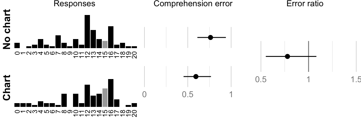

Additional Analysis

Bias in responses

cat("Mean response no-chart: ", format_ci(meanCI.bootstrap(num_nograph), sigdigits = 3), 
    "\n")

## Mean response no-chart:  11.3, CI [10.2, 12.2]

cat("Mean response chart:    ", format_ci(meanCI.bootstrap(num_graph), sigdigits = 3), 
    "\n")

## Mean response chart:     11.8, CI [10.7, 12.7]

cat("Mean difference:        ", format_ci(diffMeanCI.bootstrap(num_graph, num_nograph)), 
    "\n")

## Mean difference:         0.48, CI [-0.91, 1.85]

Experiment 4

# Clean up memory
rm(list = ls())

# Experiment filenames
results_file <- "exp4/results"
mturk_file <- "exp4/mturk"
invalid_answers_file <- "exp4/invalid_answers"
figure_path <- "plots/exp4-"

# Stimuli values (used to compute comprehension errors)
control <- 83  # % sick people without the drug
drug <- 63  # % sick people with the drug
# compute the true answer given the data
true_answer <- 63/83 * 20

# Values reported by Tal and Wanksink to add to our plots as a comparison
bws_nochart <- 4.66
bws_chart <- 5.75
bws_p <- 0.0066

Planned Analysis

library("plyr")
library("dplyr")

source("CI.helpers.R")
source("misc.helpers.R")
source("plotting functions.R")

# indicated whether we want ggplot to save the generated plots
save_plots <- FALSE
# print plots to screen
print_plots <- TRUE

Load data

# Load experiment data from csv file

if (exists("results_file")) {
    data <- read.csv(paste("data/", results_file, ".csv", sep = ""), sep = ",")
}

# Add crowdflower metadata (if exists)

if (exists("crowflower_file")) {
    crowdsourcedata <- read.csv(paste("data/", crowflower_file, ".csv", sep = ""), 
        sep = ",")
    data$code <- as.character(data$code)
    crowdsourcedata$completion_code <- as.character(crowdsourcedata$completion_code)
    data <- left_join(data, crowdsourcedata, by = c(code = "completion_code"))
    
    # Load country codes
    country_file <- "countries"
    countrydata <- read.csv(paste("data/", country_file, ".csv", sep = ""), 
        sep = ",")
}

# Add mturk metadata (if exists)

if (exists("mturk_file")) {
    crowdsourcedata <- read.csv(paste("data/", mturk_file, ".csv", sep = ""), 
        sep = ",")
    data$code <- as.character(data$code)
    crowdsourcedata$Answer.completion_code <- as.character(crowdsourcedata$Answer.completion_code)
    data <- left_join(data, crowdsourcedata, by = c(code = "Answer.completion_code"))
}

Invalid jobs

# Utility function for printing percentages
percent <- function(x, n) {
    if (x/n < 0.01) 
        r <- 1 else r <- 0
    paste(" (", format_number(100 * x/n, r), "%)", sep = "")
}

data_invalid <- read.csv(paste("data/", invalid_answers_file, ".csv", sep = ""), 
    sep = ",")
n_valid <- nrow(data)
n_invalid <- nrow(data_invalid)
n <- n_valid + n_invalid
cat("Valid jobs:   ", n_valid, "\n")

## Valid jobs:    160

cat("Invalid jobs: ", n_invalid, "\n\n")

## Invalid jobs:  29

# 
n_failed_attention <- nrow(data_invalid[data_invalid$test_question != "common_cold", 
    ])
n_abnormal_time <- nrow(data_invalid[data_invalid$time_taken < 30 | data_invalid$time_taken > 
    15 * 60, ])
n_previous_study <- nrow(data_invalid[data_invalid$previous_study == "yes", 
    ])
cat("Failed attention check:   ", n_failed_attention, percent(n_failed_attention, 
    n), "\n", sep = "")

## Failed attention check:   6 (3%)

cat("Abnormal completion time: ", n_abnormal_time, percent(n_abnormal_time, 
    n), "\n", sep = "")

## Abnormal completion time: 0 (0%)

cat("Did study before:         ", n_previous_study, percent(n_previous_study, 
    n), "\n", sep = "")

## Did study before:         0 (0%)

Sample size, completion time and demographics

print.title("Participants")

## 
## ###################################
## # Participants 
## ###################################

# Sample size

N <- nrow(data)
cat("Total sample size:  ", N, "\n")

## Total sample size:   160

cat("n =", sum(data$condition == "no_graph"), "for the no-chart condition\n")

## n = 80 for the no-chart condition

cat("n =", sum(data$condition == "graph"), "for the chart condition\n\n")

## n = 80 for the chart condition

# Job completion time

mt <- median(data$time_taken)
cat("Median job completion time:", format_number(mt/60, 2), "minutes.\n\n")

## Median job completion time: 1.7 minutes.

# Countries

if (exists("crowflower_file")) {
    data$country <- sapply(data$X_country, function(code) countrydata$name[match(code, 
        countrydata$alpha.3)])
    data$subregion <- sapply(data$X_country, function(code) countrydata$sub.region[match(code, 
        countrydata$alpha.3)])
    data$continent <- sapply(data$X_country, function(code) countrydata$region[match(code, 
        countrydata$alpha.3)])
    cat("Number of different countries:", length(unique(data$country)), "\n")
    print.percents(data$continent)
}

# Gender distribution

# Column is present in all but experiment 3
if ("gender" %in% colnames(data)) {
    cat("\nGender:\n")
    print.percents(data$gender)
}

## 
## Gender:
##              n  %
## 1      male 89 56
## 2    female 70 44
## 3 no_answer  1  1

# Age

# Column is present in all but experiment 3
if ("age" %in% colnames(data)) {
    cat("\nMean age:", round(mean(data$age)), "\n")
}

## 
## Mean age: 37

# Education

# Column is present in all but experiment 3
if ("education" %in% colnames(data)) {
    cat("\nEducation:\n")
    print.percents(data$education)
}

## 
## Education:
##                    n  %
## 1 college_or_more 77 48
## 2    some_college 60 38
## 3     high-school 23 14

Analysis of dependent variables

##### Retrieve data

# Extract judgments of drug efficacy (values between 1 and 9).  Experiment 1
# and experiments 2-4 use different question wordings, hence we look at two
# possible columns.

# Column is present in experiment 1, which replicates the question from BwS
# experiment 1
if ("effectiveness" %in% colnames(data)) {
    eff_nograph <- data[data$condition == "no_graph", ]$effectiveness
    eff_graph <- data[data$condition == "graph", ]$effectiveness
    variable_name <- "Perceived effectiveness"
}

# Column is present in experiments 2-4, which replicate the question from
# BwS experiment 2
if ("believe_in_effectiveness" %in% colnames(data)) {
    eff_nograph <- data[data$condition == "no_graph", ]$believe_in_effectiveness
    eff_graph <- data[data$condition == "graph", ]$believe_in_effectiveness
    variable_name <- "Belief in efficacy"
}

# Extract belief in drug from the second question (yes = not effective, no =
# effective).

# Column is present in experiment 1 only.
if ("reduces_sickness" %in% colnames(data)) {
    yesno_to_01 <- function(x) {
        if (x == "yes") 
            1 else if (x == "no") 
            0 else NA
    }
    ill_nograph <- data[data$condition == "no_graph", ]$reduces_sickness
    ill_graph <- data[data$condition == "graph", ]$reduces_sickness
    ill_nograph <- sapply(ill_nograph, yesno_to_01)
    ill_graph <- sapply(ill_graph, yesno_to_01)
}

# Extract answers to comprehension question

num_nograph <- data[data$condition == "no_graph", ]$comprehension
num_graph <- data[data$condition == "graph", ]$comprehension

Belief in Efficacy

##### CIs for judgment of efficacy on a 1--9 scale

mean_eff_nograph <- meanCI.bootstrap(eff_nograph)
mean_eff_graph <- meanCI.bootstrap(eff_graph)
mean_eff_diff <- diffMeanCI.bootstrap(eff_graph, eff_nograph)

print.title(variable_name)

## 
## ###################################
## # Belief in efficacy 
## ###################################

cat("Mean efficacy no-chart: ", format_ci(mean_eff_nograph), "\n")

## Mean efficacy no-chart:  6.8, CI [6.6, 7.1]

cat("Mean efficacy chart:    ", format_ci(mean_eff_graph), "\n")

## Mean efficacy chart:     5.9, CI [5.5, 6.3]

cat("Difference:             ", format_ci(mean_eff_diff), "\n")

## Difference:              -0.92, CI [-1.42, -0.50]

# NHST version for comparison (used in the original paper, but not part of
# this planned analysis)

ttest <- t.test(eff_graph, eff_nograph)
mean_eff_diff_normal <- c(mean(eff_graph) - mean(eff_nograph), ttest$conf.int[1], 
    ttest$conf.int[2])
cat("(using a t-test)        ", format_ci(mean_eff_diff_normal), "p =", format_number(ttest$p.value), 
    "\n")

## (using a t-test)         -0.92, CI [-1.39, -0.46] p = 0.00013

# Display distributions of efficacy judgments and confidence intervals for
# estimates

## compile CIs and BwS results into a dataframe for plotting
eff_df <- NULL
eff_df <- add.ci.to.df(mean_eff_nograph, "no chart", "ours", eff_df)
eff_df <- add.ci.to.df(c(bws_nochart, bws_nochart, bws_nochart), "no chart", 
    "BwS", eff_df)
eff_df <- add.ci.to.df(mean_eff_graph, "chart", "ours", eff_df)
eff_df <- add.ci.to.df(c(bws_chart, bws_chart, bws_chart), "chart", "BwS", eff_df)

eff_diff_df <- NULL
eff_diff_df <- add.ci.to.df(mean_eff_diff, " ", "ours")
eff_diff_df <- add.ci.to.df(ci_from_p(bws_chart - bws_nochart, bws_p), " ", 
    "BwS", eff_diff_df)

if (variable_name == "Belief in efficacy") {
    # plotting for experiments 2-4
    eff.hist.no_chart <- histo(eff_nograph, 9, "no chart", 0, 1)
    eff.hist.chart <- histo(eff_graph, 9, "chart", 0, 1)
    
    eff.cis <- perceived.effectiveness.ciplot(eff_df, eff_diff_df)
    
    plot <- drawVertical(eff.hist.no_chart, eff.hist.chart, eff.cis, name.eff.exp24, 
        "Difference")
    if (save_plots) 
        save_plot(paste(sep = "", figure_path, "believe_in_efficacy_plot.pdf"), 
            plot, base_aspect_ratio = 3, base_height = 2)
    if (print_plots) 
        print(plot)
    
} else {
    # plotting for experiment 1
    eff.hist.no_chart <- histo(eff_nograph, 9, "no chart", 0, 1)
    eff.hist.chart <- histo(eff_graph, 9, "chart", 0, 1)
    eff.cis <- perceived.effectiveness.1.ciplot(eff_df, eff_diff_df)
    
    plot <- drawVertical(eff.hist.no_chart, eff.hist.chart, eff.cis, name.eff.exp1, 
        "Difference")
    if (save_plots) 
        save_plot(paste(sep = "", figure_path, "perceived_effectiveness_plot.pdf"), 
            plot, base_aspect_ratio = 3, base_height = 2)
    if (print_plots) 
        print(plot)
}

##### CIs for binary belief in efficacy

# Column is present in experiment 1 only, as subsequent experiments didn't
# include that question.
if ("reduces_sickness" %in% colnames(data)) {
    
    mean_ill_nograph <- propCI(sum(ill_nograph == 1), length(ill_nograph))
    mean_ill_graph <- propCI(sum(ill_graph == 1), length(ill_graph))
    mean_ill_diff <- diffpropCI(sum(ill_graph == 1), length(ill_graph), sum(ill_nograph == 
        1), length(ill_nograph))
    
    print.title("Belief in efficacy (binary)")
    cat("Proportion of 'yes' no-chart: ", format_ci(mean_ill_nograph, percent = TRUE), 
        "\n")
    cat("Proportion of 'yes' chart:    ", format_ci(mean_ill_graph, percent = TRUE), 
        "\n")
    cat("Difference:                   ", format_ci(mean_ill_diff, percent = TRUE), 
        "\n")
    
    # NHST version for comparison (used in the original paper, but not part of
    # this planned analysis)
    
    yes <- c(sum(ill_graph == 1), sum(ill_nograph == 1))
    all <- c(length(ill_graph), length(ill_nograph))
    proptest <- prop.test(yes, all, correct = F)  # disable continuity correction to get the same p-value
    mean_ill_diff_2 <- c(yes[1]/all[1] - yes[2]/all[2], proptest$conf.int[1], 
        proptest$conf.int[2])
    cat("(using an X-squared test)     ", format_ci(mean_ill_diff_2, percent = TRUE), 
        "p =", format_number(proptest$p.value), "\n")
    
    # Plot our results in comparison to the BwS results
    
    # Tal and Wanksink's results
    bws.cis.no_graph <- propCI(21, 31)
    bws.cis.graph <- propCI(28, 29)
    bws.cis.diff <- diffpropCI(28, 29, 21, 31)
    
    # construct the dataframes for plotting
    efficiency.df <- NULL
    efficiency.df <- add.ci.to.df(mean_ill_nograph, "no chart", "ours", efficiency.df)
    efficiency.df <- add.ci.to.df(mean_ill_graph, "chart", "ours", efficiency.df)
    efficiency.df <- add.ci.to.df(bws.cis.no_graph, "no chart", "BwS", efficiency.df)
    efficiency.df <- add.ci.to.df(bws.cis.graph, "chart", "BwS", efficiency.df)
    
    efficiency.diff.df <- NULL
    efficiency.diff.df <- add.ci.to.df(mean_ill_diff, " ", "ours", efficiency.diff.df)
    efficiency.diff.df <- add.ci.to.df(bws.cis.diff, " ", "BwS", efficiency.diff.df)
    
    # plot
    efficiency.ciplot <- efficacy.belief.ciplot(efficiency.df, efficiency.diff.df)
    efficiency.plot <- drawHorizontalEfficiency(efficiency.ciplot, "Belief in efficacy", 
        "Difference")
    if (save_plots) 
        save_plot(paste(sep = "", figure_path, "belief_in_efficacy_plot.pdf"), 
            efficiency.plot, base_aspect_ratio = 4, base_height = 1.5)
    if (print_plots) 
        print(efficiency.plot)
}

Comprehension question

# Display distributions of comprehension test responses

# par(mfrow=c(1,2)) myhist('Number sick - no chart', num_nograph, 0, 20, 15)
# myhist('Number sick - chart', num_graph, 0, 20, 15)

#### CIs for errors at the comprehension question

# Define error
psick <- drug/control
logodds <- function(p) {
    log(p/(1 - p))
}
logodds.psick <- logodds(psick)
error <- function(n) {
    n[n == 0] <- 0.1
    n[n == 20] <- 19.9
    abs(logodds(n/20) - logodds.psick)
}

# Compute errors
data$error <- error(data$comprehension)
err_nograph <- error(num_nograph)
err_graph <- error(num_graph)

# Use geometric mean to reduce the influence of outliers and increase the
# weight of close-to-exact answers
mean_err_nograph <- geomMeanCI.bootstrap(err_nograph)
mean_err_graph <- geomMeanCI.bootstrap(err_graph)
mean_err_diff <- ratioGeomMeanCI.bootstrap(err_graph, err_nograph)
print.title("Comprehension error")

## 
## ###################################
## # Comprehension error 
## ###################################

cat("Geometric mean error no-chart: ", format_ci(mean_err_nograph), "\n")

## Geometric mean error no-chart:  0.47, CI [0.36, 0.60]

cat("Geometric mean error chart:    ", format_ci(mean_err_graph), "\n")

## Geometric mean error chart:     0.46, CI [0.35, 0.59]

cat("Ratio:                         ", format_ci(mean_err_diff), "\n")

## Ratio:                          0.97, CI [0.69, 1.42]

# Plot raw responses and confidence intervals

comp.hist.no_chart <- histo(num_nograph, 20, "no chart", true_answer, 1)
comp.hist.chart <- histo(num_graph, 20, "chart", true_answer, 1)

# construct the dataframes for plotting
comprehension.df <- NULL
comprehension.df <- add.ci.to.df(mean_err_nograph, "no chart", "ours", comprehension.df)
comprehension.df <- add.ci.to.df(mean_err_graph, "chart", "ours", comprehension.df)

comprehension.diff.df <- NULL
comprehension.diff.df <- add.ci.to.df(mean_err_diff, " ", "ours", comprehension.diff.df)

# plot
comp.cis <- comprehension.ciplot(comprehension.df, comprehension.diff.df)
comp.plot <- drawVerticalComp(comp.hist.no_chart, comp.hist.chart, comp.cis, 
    "Comprehension error", "Error ratio")
if (save_plots) save_plot(paste(sep = "", figure_path, "comprehension_plot.pdf"), 
    comp.plot, base_aspect_ratio = 3, base_height = 2)
if (print_plots) print(comp.plot)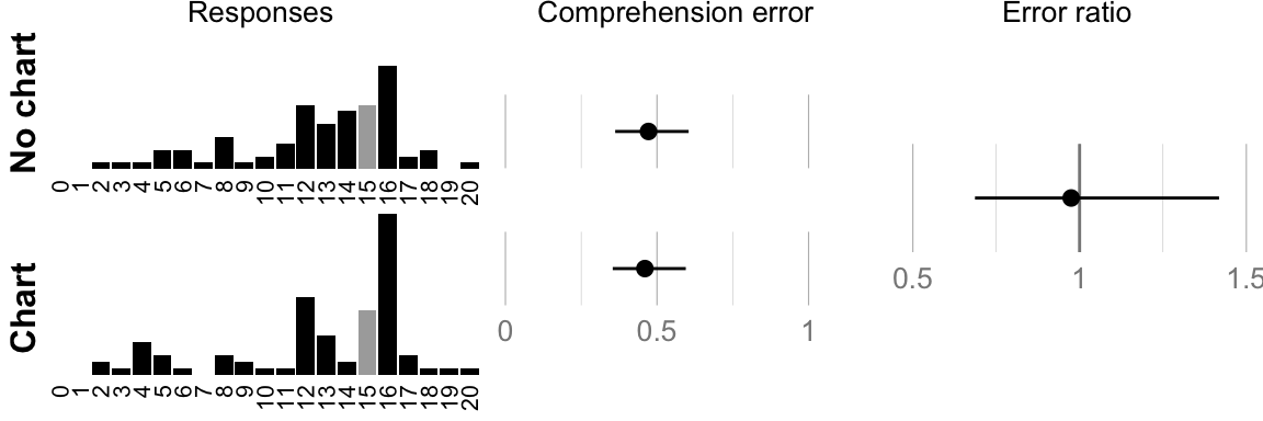

Extra planned analysis

# Remove NAs for belief in science (not sure how this happened)
data_clean <- data[!is.na(data$belief_in_science), ]

# Break down by condition
nograph <- data_clean[data_clean$condition == "no_graph", ]
graph <- data_clean[data_clean$condition == "graph", ]

# Datasets with positively polarized people removed
nograph_nopp <- nograph[nograph$belief_in_medicine < 7, ]
graph_nopp <- graph[graph$belief_in_medicine < 7, ]

# Keep the removed people to plot separately
nograph_removed <- nograph[nograph$belief_in_medicine >= 7, ]
graph_removed <- graph[graph$belief_in_medicine >= 7, ]

# Function for computing and plotting the regression
fit <- function(title, x, xs, y, ys, x_ignored = NULL, y_ignored = NULL) {
    coeff_bigger = 1.2
    exponent = 0.5
    AA = xyTable(x, y)
    plot(AA$x, AA$y, main = title, xlab = xs, ylab = ys, xlim = c(1, 9), xaxp = c(1, 
        9, 8), ylim = c(1, 9), yaxp = c(1, 9, 8), yaxs = "r", type = "n")
    
    fit <- lm(y ~ x)
    clip(min(AA$x) - 0.5, max(AA$x) + 0.5, 0, 10)
    abline(fit, lty = 1)
    clip(0, 10, 0, 10)
    confint(fit)
    
    points(AA$x, AA$y, cex = (AA$number)^exponent * coeff_bigger, col = rgb(0, 
        0, 0, 0.2), pch = 16)
    text(AA$x, AA$y, ifelse(AA$number > 1, AA$number, ""), col = rgb(0, 0, 0, 
        0.5))
    if (length(x_ignored) > 0) {
        AA = xyTable(x_ignored, y_ignored)
        points(AA$x, AA$y, cex = (AA$number)^exponent * coeff_bigger, col = rgb(0, 
            0, 0, 0.2), pch = 1)
        text(AA$x, AA$y, ifelse(AA$number > 1, AA$number, ""), col = rgb(0, 
            0, 0, 0.3))
    }
}

# Interaction between belief in science and chart persuasiveness (Fig 16
# left part)
layout(matrix(c(1, 2, 3, 4), 1, 4, byrow = T), widths = c(2.5, 2.5, 2.5, 2.5), 
    heights = c(2.5))
fit("No chart", nograph$belief_in_science, "Belief in science", nograph$believe_in_effectiveness, 
    "Belief in efficacy")
fit("Chart", graph$belief_in_science, "Belief in science", graph$believe_in_effectiveness, 
    "Belief in efficacy")

# Interaction between polarization and chart persuasiveness (Fig 16 right
# part)

fit("No chart", nograph_nopp$belief_in_medicine, "Polarization", nograph_nopp$believe_in_effectiveness, 
    "Belief in efficacy", nograph_removed$belief_in_medicine, nograph_removed$believe_in_effectiveness)
fit("Chart", graph_nopp$belief_in_medicine, "Polarization", graph_nopp$believe_in_effectiveness, 
    "Belief in efficacy", graph_removed$belief_in_medicine, graph_removed$believe_in_effectiveness)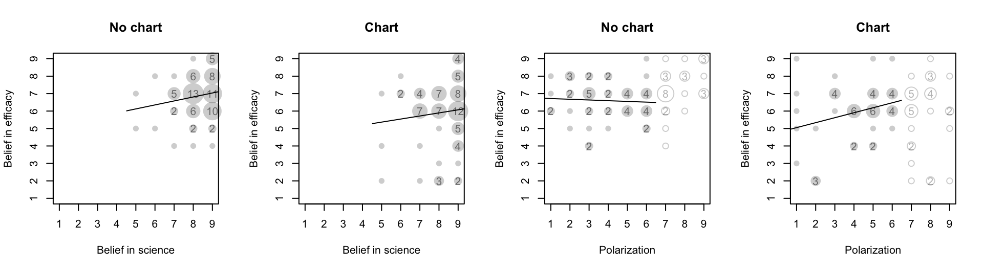

Left group: interaction betweeen belief in science and chart persuasiveness Right group: interaction between polarization and chart persuasiveness

Regression analysis

# Difference between slopes: belief in science and chart persuasiveness

cat("Difference between slopes -- belief in science:      ", format_ci(diff.slopes.bootstrap(nograph$belief_in_science, 
    nograph$believe_in_effectiveness, graph$belief_in_science, graph$believe_in_effectiveness)), 
    "\n")

## Difference between slopes -- belief in science:       -0.052, CI [-0.61, 0.37]

cat("Difference between slopes -- polarization:           ", format_ci(diff.slopes.bootstrap(nograph_nopp$belief_in_medicine, 
    nograph_nopp$believe_in_effectiveness, graph_nopp$belief_in_medicine, graph_nopp$believe_in_effectiveness)), 
    "\n")

## Warning in norm.inter(t, adj.alpha): extreme order statistics used as
## endpoints

## Difference between slopes -- polarization:            0.33, CI [0.31, 0.75]

Meta Analysis

# Clean up memory
rm(list = ls())

library("dplyr")
library("plyr")
library("bootES")

source("CI.helpers.R")
source("misc.helpers.R")

# Number of replicates to use in bootstrapping. The higher the more accurate
# the results. Warning: a large R can yield very lengthy computations.
R = 5000

######################################################################## Load data

# Read data from all 4 experiments

data1 <- read.csv(paste("data/exp1/results.csv", sep = ""), sep = ",")
data2 <- read.csv(paste("data/exp2/results.csv", sep = ""), sep = ",")
data3 <- read.csv(paste("data/exp3/results.csv", sep = ""), sep = ",")
data4 <- read.csv(paste("data/exp4/results.csv", sep = ""), sep = ",")

# Compute the total number of observations

N <- nrow(data1) + nrow(data2) + nrow(data3) + nrow(data4)
cat("Total sample size: N =", N, "\n\n")

## Total sample size: N = 623

######################################################################## Retrieve observations of interest

# Efficacy judgement data for all 4 experiments

eff1_nograph <- data1[data1$condition == "no_graph", ]$effectiveness
eff2_nograph <- data2[data2$condition == "no_graph", ]$believe_in_effectiveness
eff3_nograph <- data3[data3$condition == "no_graph", ]$believe_in_effectiveness
eff4_nograph <- data4[data4$condition == "no_graph", ]$believe_in_effectiveness
eff1_graph <- data1[data1$condition == "graph", ]$effectiveness
eff2_graph <- data2[data2$condition == "graph", ]$believe_in_effectiveness
eff3_graph <- data3[data3$condition == "graph", ]$believe_in_effectiveness
eff4_graph <- data4[data4$condition == "graph", ]$believe_in_effectiveness

# Comprehension error data for all 4 experiments

logodds <- function(p) {
    log(p/(1 - p))
}
error <- function(n, control, drug) {
    n[n == 0] <- 0.1
    n[n == 20] <- 19.9
    abs(logodds(n/20) - logodds(drug/control))
}
error1 <- function(n) {
    error(n, 87, 47)
}  # For exp 1
error2 <- function(n) {
    error(n, 83, 63)
}  # For exp 2,3,4

err1_nograph <- error1(data1[data1$condition == "no_graph", ]$comprehension)
err2_nograph <- error2(data2[data2$condition == "no_graph", ]$comprehension)
err3_nograph <- error2(data3[data3$condition == "no_graph", ]$comprehension)
err4_nograph <- error2(data4[data4$condition == "no_graph", ]$comprehension)
err1_graph <- error1(data1[data1$condition == "graph", ]$comprehension)
err2_graph <- error2(data2[data2$condition == "graph", ]$comprehension)
err3_graph <- error2(data3[data3$condition == "graph", ]$comprehension)
err4_graph <- error2(data4[data4$condition == "graph", ]$comprehension)

######################################################################## Compute standardized effect sizes and their CI for each experiment

# Convenience function that computes, prints and returns the standardized
# effect size for the mean difference between two independent samples, with
# its 95% BCa bootstrap CI.

printEffectSize <- function(exp_name, data_nograph, data_graph) {
    data <- data.frame(obs = c(data_nograph, data_graph), group = c(rep("nograph", 
        length(data_nograph)), rep("graph", length(data_graph))))
    set.seed(0)  # make deterministic
    b <- bootES(data, R = R, effect.type = "cohens.d", data.col = "obs", group.col = "group", 
        contrast = c(nograph = 1, graph = -1))
    pointEstimate <- b[[1]]
    bootci <- boot.ci(b, type = "bca", conf = conf.level)
    cat("Effect size for ", exp_name, ": ", format_ci(c(pointEstimate, bootci$bca[4], 
        bootci$bca[5])), "\n", sep = "")
    return(data.frame(estimate = pointEstimate, ci.low = bootci$bca[4], ci.high = bootci$bca[5]))
}

# Note: the exact point and interval estimates obtained here may differ
# slightly from the paper because in the previous version, the random seed
# was not reset before each call to bootES. Use a large value of R to get
# more accurate estimates.

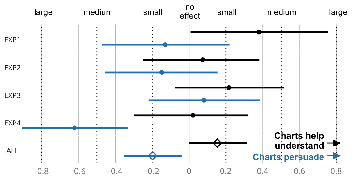
exp1.belief <- printEffectSize("exp 1 belief     ", eff1_graph, eff1_nograph)

## Effect size for exp 1 belief     : -0.13, CI [-0.47, 0.22]

exp2.belief <- printEffectSize("exp 2 belief     ", eff2_graph, eff2_nograph)

## Effect size for exp 2 belief     : -0.15, CI [-0.45, 0.15]

exp3.belief <- printEffectSize("exp 3 belief     ", eff3_graph, eff3_nograph)

## Effect size for exp 3 belief     : 0.081, CI [-0.22, 0.38]

exp4.belief <- printEffectSize("exp 4 belief     ", eff4_graph, eff4_nograph)

## Effect size for exp 4 belief     : -0.62, CI [-0.91, -0.33]

cat("\n")

exp1.error <- printEffectSize("exp 1 log error  ", log(err1_nograph), log(err1_graph))

## Effect size for exp 1 log error  : 0.38, CI [0.0084, 0.75]

exp2.error <- printEffectSize("exp 2 log error  ", log(err2_nograph), log(err2_graph))

## Effect size for exp 2 log error  : 0.075, CI [-0.25, 0.38]

exp3.error <- printEffectSize("exp 3 log error  ", log(err3_nograph), log(err3_graph))

## Effect size for exp 3 log error  : 0.22, CI [-0.078, 0.52]

exp4.error <- printEffectSize("exp 4 log error  ", log(err4_nograph), log(err4_graph))

## Effect size for exp 4 log error  : 0.022, CI [-0.30, 0.32]

cat("\n")

######################################################################## Compute the aggregated standardized effect size and its CI

# Custom function that performs a contrast weighted by sample size to
# compute a standardized effect size for all 4 experiments together, and its
# 95% BCa bootstrap CI.  ng1: no-graph condition, experiment 1 ng2: no-graph
# condition, experiment 2 ng3: no-graph condition, experiment 3 ng4:
# no-graph condition, experiment 4 g1: graph condition, experiment 1 g2:
# graph condition, experiment 2 g3: graph condition, experiment 3 g4: graph
# condition, experiment 4

printMetaEffectSize <- function(exp, ng1, ng2, ng3, ng4, g1, g2, g3, g4) {
    
    # Create custom data frame to hold all the data
    data <- data.frame(obs = c(ng1, ng2, ng3, ng4, g1, g2, g3, g4), group = c(rep("ng1", 
        length(ng1)), rep("ng2", length(ng2)), rep("ng3", length(ng3)), rep("ng4", 
        length(ng4)), rep("g1", length(g1)), rep("g2", length(g2)), rep("g3", 
        length(g3)), rep("g4", length(g4))))
    
    # Set weights for the contrast
    n_ng = length(ng1) + length(ng2) + length(ng3) + length(ng4)  # total sample size for no-graph
    n_g = length(g1) + length(g2) + length(g3) + length(g4)  # total sample size for graph
    w_ng1 = length(ng1)/n_ng
    w_ng2 = length(ng2)/n_ng
    w_ng3 = length(ng3)/n_ng
    w_ng4 = length(ng4)/n_ng
    w_g1 = length(g1)/n_g
    w_g2 = length(g2)/n_g
    w_g3 = length(g3)/n_g
    w_g4 = length(g4)/n_g
    # print(w_ng1+w_ng2+w_ng3-w_g1-w_g2-w_g3) # should be zero
    
    set.seed(0)  # make deterministic
    b <- bootES(data, R = R, effect.type = "cohens.d", data.col = "obs", group.col = "group", 
        scale.weights = T, contrast = c(ng1 = w_ng1, ng2 = w_ng2, ng3 = w_ng3, 
            ng4 = w_ng4, g1 = -w_g1, g2 = -w_g2, g3 = -w_g3, g4 = -w_g4))
    pointEstimate <- b[[1]]
    bootci <- boot.ci(b, type = "bca", conf = conf.level)
    cat("Effect size for ", exp, ": ", format_ci(c(pointEstimate, bootci$bca[4], 
        bootci$bca[5])), "\n", sep = "")
    return(data.frame(estimate = pointEstimate, ci.low = bootci$bca[4], ci.high = bootci$bca[5]))
}

# Note: the exact point and interval estimates obtained here may differ
# slightly from the paper because in the previous version, the random seed
# was not reset before each call to bootES. Use a large value of R to get
# more accurate estimates.

meta.belief <- printMetaEffectSize("all belief     ", eff1_graph, eff2_graph, 
    eff3_graph, eff4_graph, eff1_nograph, eff2_nograph, eff3_nograph, eff4_nograph)

## Effect size for all belief     : -0.20, CI [-0.35, -0.040]

cat("\n")

meta.error <- printMetaEffectSize("all log error  ", log(err1_nograph), log(err2_nograph), 
    log(err3_nograph), log(err4_nograph), log(err1_graph), log(err2_graph), 
    log(err3_graph), log(err4_graph))

## Effect size for all log error  : 0.15, CI [-0.0022, 0.31]

library('ggplot2')
library("gridExtra")
library("cowplot")
source("CI.helpers.R")
source("misc.helpers.R")


scale.min <- -0.92
scale.max <- 0.82
effect.size.indicator.color <- "black"



meta.ci.df <- NULL
meta.ci.df <- add.ci.to.df(exp1.belief, "belief", "EXP1", meta.ci.df)
meta.ci.df <- add.ci.to.df(exp1.error, "error", "EXP1", meta.ci.df)
meta.ci.df <- add.ci.to.df(exp2.belief, "belief", "EXP2", meta.ci.df)
meta.ci.df <- add.ci.to.df(exp2.error, "error", "EXP2", meta.ci.df)
meta.ci.df <- add.ci.to.df(exp3.belief, "belief", "EXP3", meta.ci.df)
meta.ci.df <- add.ci.to.df(exp3.error, "error", "EXP3", meta.ci.df)
meta.ci.df <- add.ci.to.df(exp4.belief, "belief", "EXP4", meta.ci.df)
meta.ci.df <- add.ci.to.df(exp4.error, "error", "EXP4", meta.ci.df)
meta.ci.df <- add.ci.to.df(meta.belief, "belief", "ALL", meta.ci.df)
meta.ci.df <- add.ci.to.df(meta.error, "error", "ALL", meta.ci.df)




citheme <- theme_bw(base_family = "Open Sans") +
  theme( # remove the vertical grid lines
    plot.background = element_blank(),
    plot.margin = margin(t = 0, r = 0, b = 0, l = 0, unit = "pt"),
    legend.position = "none", #c(0.2,0.88),
    legend.title = element_blank(),
    legend.margin = margin(t = 0, r = 0, b = 0, l = 0, unit = "pt"),
    legend.text = element_text(size=8),
    legend.key.size = unit(c(3.5, 3.5),'mm'),
    legend.key.width = unit(c(0.3, 0.3),'cm'),
    axis.title.y = element_blank(),
    axis.title.x = element_blank(),
    axis.text.y = element_blank(),
    axis.text.x = element_text(size=10, colour="#888888", margin = margin(1,1.5,0,0,"mm")),
    panel.spacing = unit(0, "lines"),
    panel.border = element_blank(), 
    axis.line = element_blank(),
    axis.ticks = element_blank(),
    axis.line.x = element_blank(),
    panel.grid.minor.x = element_blank(),
    panel.grid.major.x = element_line(size=0.2, color="#BBBBBB"),
    panel.grid.major.y = element_blank(),
    strip.background = element_blank(),
    strip.text.y = element_text(angle = 180, margin = margin(1,-7,0,0,"mm"))
  )

condFatten <- function(x,...) {
  ifelse(x=="ALL", 1.3, 1)
}

condShape <- function(x,...) {
  ifelse(x=="ALL", 5, 16)
}

meta.ciplot <- function(df, scale = T) {

  ratioPlot <- ggplot(data= df) +
    expand_limits( y=c(scale.min, scale.max)) +
    citheme +
    geom_hline(yintercept = -0.8, color = effect.size.indicator.color, linetype = "dotted") +
    geom_hline(yintercept = -0.5, color = effect.size.indicator.color, linetype = "dotted") +
    geom_hline(yintercept = -0.2, color = effect.size.indicator.color, linetype = "dotted") +
    geom_hline(yintercept = 0, color = "black") +
    geom_hline(yintercept = 0.2, color = effect.size.indicator.color, linetype = "dotted") +
    geom_hline(yintercept = 0.5, color = effect.size.indicator.color, linetype = "dotted") +
    geom_hline(yintercept = 0.8, color = effect.size.indicator.color, linetype = "dotted") +
    coord_flip() +
    geom_pointrange(aes(y = estimate, x=reorder(name, order), ymin= ci.low, ymax = ci.high, color = name), size = condFatten(df$study), fatten = 2, shape= condShape(df$study)) +
    scale_colour_manual(name = 'belief in blue', values = setNames(c('#2b83ba', "black", "black", "black"),c("belief", "error", "meta", "afake"))) +
      geom_path(data=data.frame(name=c("error", "error", "belief", "belief"), estimate = c(0.75, 0.82, 0.75, 0.82), study= c("ALL", "ALL", "ALL", "ALL")), aes(x = name, y = estimate, color=name), arrow=arrow(angle = 25, length = unit(3, "mm"), type="closed")) +
    facet_grid(study ~ ., space= "free_x", switch = "y") +
    labs(x=NULL, y=NULL) +
    theme(axis.text.y = element_blank()) +
    scale_y_continuous(breaks= seq(from=-0.8, to=0.8, by= 0.2), labels = seq(from=-0.8, to=0.8, by= 0.2), limits = c(scale.min, scale.max))
  if (!scale) {
    ratioPlot <- ratioPlot + theme(axis.text.x = element_blank() )
  }
  return(ratioPlot)
}

metaplot <- meta.ciplot(meta.ci.df)

finalplot <- ggdraw() + 
  draw_plot(metaplot, 0, 0, 1, 0.86) +
  draw_label("large", 0.115, 0.95, vjust=1, hjust = 0.5, size = 10) +
  draw_label("medium", 0.27, 0.95, vjust=1, hjust = 0.5, size = 10) +
  draw_label("small", 0.425, 0.95, vjust=1, hjust = 0.5, size = 10) +
  draw_label("no\neffect", 0.53, 0.98, vjust=1, hjust = 0.5, size = 10) +
  draw_label("small", 0.635, 0.95, vjust=1, hjust = 0.5, size = 10) +
  draw_label("medium", 0.79, 0.95, vjust=1, hjust = 0.5, size = 10) +
  draw_label("large", 0.95, 0.95, vjust=1, hjust = 0.5, size = 10) +
 draw_label("Charts help\nunderstand", 0.91, 0.06, vjust = -1, hjust = 1, size = 11, fontface = "bold") +
  draw_label("Charts persuade", 0.91, 0.05, vjust = -1, hjust = 1, size = 11, colour = '#2b83ba', fontface = "bold")

## Warning in grid.Call(L_textBounds, as.graphicsAnnot(x$label), x$x, x$y, :
## font family 'Open Sans' not found in PostScript font database

## Warning in grid.Call(L_textBounds, as.graphicsAnnot(x$label), x$x, x$y, :
## font family 'Open Sans' not found in PostScript font database

## Warning in grid.Call(L_textBounds, as.graphicsAnnot(x$label), x$x, x$y, :
## font family 'Open Sans' not found in PostScript font database

## Warning in grid.Call(L_textBounds, as.graphicsAnnot(x$label), x$x, x$y, :
## font family 'Open Sans' not found in PostScript font database

## Warning in grid.Call(L_textBounds, as.graphicsAnnot(x$label), x$x, x$y, :
## font family 'Open Sans' not found in PostScript font database

## Warning in grid.Call(L_textBounds, as.graphicsAnnot(x$label), x$x, x$y, :
## font family 'Open Sans' not found in PostScript font database

## Warning in grid.Call(L_textBounds, as.graphicsAnnot(x$label), x$x, x$y, :
## font family 'Open Sans' not found in PostScript font database

## Warning in grid.Call(L_textBounds, as.graphicsAnnot(x$label), x$x, x$y, :
## font family 'Open Sans' not found in PostScript font database

## Warning in grid.Call(L_textBounds, as.graphicsAnnot(x$label), x$x, x$y, :
## font family 'Open Sans' not found in PostScript font database

## Warning in grid.Call(L_textBounds, as.graphicsAnnot(x$label), x$x, x$y, :
## font family 'Open Sans' not found in PostScript font database

## Warning in grid.Call(L_textBounds, as.graphicsAnnot(x$label), x$x, x$y, :
## font family 'Open Sans' not found in PostScript font database

## Warning in grid.Call(L_textBounds, as.graphicsAnnot(x$label), x$x, x$y, :
## font family 'Open Sans' not found in PostScript font database

## Warning in grid.Call(L_textBounds, as.graphicsAnnot(x$label), x$x, x$y, :
## font family 'Open Sans' not found in PostScript font database

## Warning in grid.Call(L_textBounds, as.graphicsAnnot(x$label), x$x, x$y, :
## font family 'Open Sans' not found in PostScript font database

## Warning in grid.Call(L_textBounds, as.graphicsAnnot(x$label), x$x, x$y, :
## font family 'Open Sans' not found in PostScript font database

## Warning in grid.Call(L_textBounds, as.graphicsAnnot(x$label), x$x, x$y, :
## font family 'Open Sans' not found in PostScript font database

## Warning in grid.Call(L_textBounds, as.graphicsAnnot(x$label), x$x, x$y, :
## font family 'Open Sans' not found in PostScript font database

## Warning in grid.Call(L_textBounds, as.graphicsAnnot(x$label), x$x, x$y, :
## font family 'Open Sans' not found in PostScript font database

## Warning in grid.Call(L_textBounds, as.graphicsAnnot(x$label), x$x, x$y, :
## font family 'Open Sans' not found in PostScript font database

## Warning in grid.Call(L_textBounds, as.graphicsAnnot(x$label), x$x, x$y, :
## font family 'Open Sans' not found in PostScript font database

## Warning in grid.Call(L_textBounds, as.graphicsAnnot(x$label), x$x, x$y, :
## font family 'Open Sans' not found in PostScript font database

## Warning in grid.Call(L_textBounds, as.graphicsAnnot(x$label), x$x, x$y, :
## font family 'Open Sans' not found in PostScript font database

## Warning in grid.Call(L_textBounds, as.graphicsAnnot(x$label), x$x, x$y, :
## font family 'Open Sans' not found in PostScript font database

## Warning in grid.Call(L_textBounds, as.graphicsAnnot(x$label), x$x, x$y, :
## font family 'Open Sans' not found in PostScript font database

## Warning in grid.Call(L_textBounds, as.graphicsAnnot(x$label), x$x, x$y, :
## font family 'Open Sans' not found in PostScript font database

## Warning in grid.Call(L_textBounds, as.graphicsAnnot(x$label), x$x, x$y, :
## font family 'Open Sans' not found in PostScript font database

## Warning in grid.Call(L_textBounds, as.graphicsAnnot(x$label), x$x, x$y, :
## font family 'Open Sans' not found in PostScript font database

## Warning in grid.Call(L_textBounds, as.graphicsAnnot(x$label), x$x, x$y, :
## font family 'Open Sans' not found in PostScript font database

## Warning in grid.Call(L_textBounds, as.graphicsAnnot(x$label), x$x, x$y, :
## font family 'Open Sans' not found in PostScript font database

## Warning in grid.Call(L_textBounds, as.graphicsAnnot(x$label), x$x, x$y, :
## font family 'Open Sans' not found in PostScript font database

## Warning in grid.Call(L_textBounds, as.graphicsAnnot(x$label), x$x, x$y, :
## font family 'Open Sans' not found in PostScript font database

## Warning in grid.Call(L_textBounds, as.graphicsAnnot(x$label), x$x, x$y, :
## font family 'Open Sans' not found in PostScript font database

## Warning in grid.Call(L_textBounds, as.graphicsAnnot(x$label), x$x, x$y, :
## font family 'Open Sans' not found in PostScript font database

## Warning in grid.Call(L_textBounds, as.graphicsAnnot(x$label), x$x, x$y, :
## font family 'Open Sans' not found in PostScript font database

## Warning in grid.Call(L_textBounds, as.graphicsAnnot(x$label), x$x, x$y, :
## font family 'Open Sans' not found in PostScript font database

## Warning in grid.Call(L_textBounds, as.graphicsAnnot(x$label), x$x, x$y, :
## font family 'Open Sans' not found in PostScript font database

## Warning in grid.Call(L_textBounds, as.graphicsAnnot(x$label), x$x, x$y, :
## font family 'Open Sans' not found in PostScript font database

## Warning in grid.Call(L_textBounds, as.graphicsAnnot(x$label), x$x, x$y, :
## font family 'Open Sans' not found in PostScript font database

## Warning in grid.Call(L_textBounds, as.graphicsAnnot(x$label), x$x, x$y, :
## font family 'Open Sans' not found in PostScript font database

## Warning in grid.Call(L_textBounds, as.graphicsAnnot(x$label), x$x, x$y, :
## font family 'Open Sans' not found in PostScript font database

## Warning in grid.Call(L_textBounds, as.graphicsAnnot(x$label), x$x, x$y, :
## font family 'Open Sans' not found in PostScript font database

## Warning in grid.Call(L_textBounds, as.graphicsAnnot(x$label), x$x, x$y, :
## font family 'Open Sans' not found in PostScript font database

## Warning in grid.Call(L_textBounds, as.graphicsAnnot(x$label), x$x, x$y, :
## font family 'Open Sans' not found in PostScript font database

## Warning in grid.Call(L_textBounds, as.graphicsAnnot(x$label), x$x, x$y, :
## font family 'Open Sans' not found in PostScript font database

## Warning in grid.Call(L_textBounds, as.graphicsAnnot(x$label), x$x, x$y, :
## font family 'Open Sans' not found in PostScript font database

## Warning in grid.Call(L_textBounds, as.graphicsAnnot(x$label), x$x, x$y, :
## font family 'Open Sans' not found in PostScript font database

## Warning in grid.Call(L_textBounds, as.graphicsAnnot(x$label), x$x, x$y, :
## font family 'Open Sans' not found in PostScript font database

## Warning in grid.Call(L_textBounds, as.graphicsAnnot(x$label), x$x, x$y, :
## font family 'Open Sans' not found in PostScript font database

## Warning in grid.Call(L_textBounds, as.graphicsAnnot(x$label), x$x, x$y, :
## font family 'Open Sans' not found in PostScript font database

## Warning in grid.Call(L_textBounds, as.graphicsAnnot(x$label), x$x, x$y, :
## font family 'Open Sans' not found in PostScript font database

## Warning in grid.Call(L_textBounds, as.graphicsAnnot(x$label), x$x, x$y, :
## font family 'Open Sans' not found in PostScript font database

## Warning in grid.Call(L_textBounds, as.graphicsAnnot(x$label), x$x, x$y, :
## font family 'Open Sans' not found in PostScript font database

## Warning in grid.Call(L_textBounds, as.graphicsAnnot(x$label), x$x, x$y, :
## font family 'Open Sans' not found in PostScript font database

## Warning in grid.Call(L_textBounds, as.graphicsAnnot(x$label), x$x, x$y, :
## font family 'Open Sans' not found in PostScript font database

## Warning in grid.Call(L_textBounds, as.graphicsAnnot(x$label), x$x, x$y, :
## font family 'Open Sans' not found in PostScript font database

## Warning in grid.Call(L_textBounds, as.graphicsAnnot(x$label), x$x, x$y, :
## font family 'Open Sans' not found in PostScript font database

## Warning in grid.Call(L_textBounds, as.graphicsAnnot(x$label), x$x, x$y, :
## font family 'Open Sans' not found in PostScript font database

## Warning in grid.Call(L_textBounds, as.graphicsAnnot(x$label), x$x, x$y, :
## font family 'Open Sans' not found in PostScript font database

## Warning in grid.Call(L_textBounds, as.graphicsAnnot(x$label), x$x, x$y, :
## font family 'Open Sans' not found in PostScript font database

## Warning in grid.Call(L_textBounds, as.graphicsAnnot(x$label), x$x, x$y, :
## font family 'Open Sans' not found in PostScript font database

## Warning in grid.Call(L_textBounds, as.graphicsAnnot(x$label), x$x, x$y, :
## font family 'Open Sans' not found in PostScript font database

## Warning in grid.Call(L_textBounds, as.graphicsAnnot(x$label), x$x, x$y, :
## font family 'Open Sans' not found in PostScript font database

## Warning in grid.Call(L_textBounds, as.graphicsAnnot(x$label), x$x, x$y, :
## font family 'Open Sans' not found in PostScript font database

## Warning in grid.Call(L_textBounds, as.graphicsAnnot(x$label), x$x, x$y, :
## font family 'Open Sans' not found in PostScript font database

## Warning in grid.Call(L_textBounds, as.graphicsAnnot(x$label), x$x, x$y, :
## font family 'Open Sans' not found in PostScript font database

## Warning in grid.Call(L_textBounds, as.graphicsAnnot(x$label), x$x, x$y, :
## font family 'Open Sans' not found in PostScript font database

## Warning in grid.Call(L_textBounds, as.graphicsAnnot(x$label), x$x, x$y, :
## font family 'Open Sans' not found in PostScript font database

## Warning in grid.Call(L_textBounds, as.graphicsAnnot(x$label), x$x, x$y, :
## font family 'Open Sans' not found in PostScript font database

## Warning in grid.Call(L_textBounds, as.graphicsAnnot(x$label), x$x, x$y, :
## font family 'Open Sans' not found in PostScript font database

## Warning in grid.Call(L_textBounds, as.graphicsAnnot(x$label), x$x, x$y, :
## font family 'Open Sans' not found in PostScript font database

## Warning in grid.Call(L_textBounds, as.graphicsAnnot(x$label), x$x, x$y, :
## font family 'Open Sans' not found in PostScript font database

## Warning in grid.Call(L_textBounds, as.graphicsAnnot(x$label), x$x, x$y, :
## font family 'Open Sans' not found in PostScript font database

## Warning in grid.Call(L_textBounds, as.graphicsAnnot(x$label), x$x, x$y, :
## font family 'Open Sans' not found in PostScript font database

## Warning in grid.Call(L_textBounds, as.graphicsAnnot(x$label), x$x, x$y, :
## font family 'Open Sans' not found in PostScript font database

## Warning in grid.Call(L_textBounds, as.graphicsAnnot(x$label), x$x, x$y, :
## font family 'Open Sans' not found in PostScript font database

## Warning in grid.Call(L_textBounds, as.graphicsAnnot(x$label), x$x, x$y, :
## font family 'Open Sans' not found in PostScript font database

## Warning in grid.Call(L_textBounds, as.graphicsAnnot(x$label), x$x, x$y, :
## font family 'Open Sans' not found in PostScript font database

## Warning in grid.Call(L_textBounds, as.graphicsAnnot(x$label), x$x, x$y, :
## font family 'Open Sans' not found in PostScript font database

## Warning in grid.Call(L_textBounds, as.graphicsAnnot(x$label), x$x, x$y, :
## font family 'Open Sans' not found in PostScript font database

## Warning in grid.Call(L_textBounds, as.graphicsAnnot(x$label), x$x, x$y, :
## font family 'Open Sans' not found in PostScript font database

## Warning in grid.Call(L_textBounds, as.graphicsAnnot(x$label), x$x, x$y, :
## font family 'Open Sans' not found in PostScript font database

## Warning in grid.Call(L_textBounds, as.graphicsAnnot(x$label), x$x, x$y, :
## font family 'Open Sans' not found in PostScript font database

## Warning in grid.Call(L_textBounds, as.graphicsAnnot(x$label), x$x, x$y, :
## font family 'Open Sans' not found in PostScript font database

## Warning in grid.Call(L_textBounds, as.graphicsAnnot(x$label), x$x, x$y, :
## font family 'Open Sans' not found in PostScript font database

## Warning in grid.Call(L_textBounds, as.graphicsAnnot(x$label), x$x, x$y, :
## font family 'Open Sans' not found in PostScript font database

## Warning in grid.Call(L_textBounds, as.graphicsAnnot(x$label), x$x, x$y, :
## font family 'Open Sans' not found in PostScript font database

## Warning in grid.Call(L_textBounds, as.graphicsAnnot(x$label), x$x, x$y, :
## font family 'Open Sans' not found in PostScript font database

## Warning in grid.Call(L_textBounds, as.graphicsAnnot(x$label), x$x, x$y, :
## font family 'Open Sans' not found in PostScript font database

## Warning in grid.Call(L_textBounds, as.graphicsAnnot(x$label), x$x, x$y, :
## font family 'Open Sans' not found in PostScript font database

## Warning in grid.Call(L_textBounds, as.graphicsAnnot(x$label), x$x, x$y, :
## font family 'Open Sans' not found in PostScript font database

## Warning in grid.Call(L_textBounds, as.graphicsAnnot(x$label), x$x, x$y, :
## font family 'Open Sans' not found in PostScript font database

## Warning in grid.Call(L_textBounds, as.graphicsAnnot(x$label), x$x, x$y, :
## font family 'Open Sans' not found in PostScript font database

## Warning in grid.Call(L_textBounds, as.graphicsAnnot(x$label), x$x, x$y, :
## font family 'Open Sans' not found in PostScript font database

## Warning in grid.Call(L_textBounds, as.graphicsAnnot(x$label), x$x, x$y, :
## font family 'Open Sans' not found in PostScript font database

## Warning in grid.Call(L_textBounds, as.graphicsAnnot(x$label), x$x, x$y, :
## font family 'Open Sans' not found in PostScript font database

## Warning in grid.Call(L_textBounds, as.graphicsAnnot(x$label), x$x, x$y, :
## font family 'Open Sans' not found in PostScript font database

## Warning in grid.Call(L_textBounds, as.graphicsAnnot(x$label), x$x, x$y, :
## font family 'Open Sans' not found in PostScript font database

## Warning in grid.Call(L_textBounds, as.graphicsAnnot(x$label), x$x, x$y, :
## font family 'Open Sans' not found in PostScript font database

## Warning in grid.Call(L_textBounds, as.graphicsAnnot(x$label), x$x, x$y, :
## font family 'Open Sans' not found in PostScript font database

print(finalplot)

Blinded with Science or Informed by Charts? Annotated Analysis Scripts of a Replication Study

Pierre Dragicevic and Yvonne Jansen

All scripts were first generated in March 2017, then cleaned up and marked up in August/September 2017

Experiment 1

Planned Analysis

Load data

Invalid jobs

Sample size, completion time and demographics

Analysis of dependent variables

Judgment of efficacy

Binary belief in efficacy

Comprehension question

Additional Analysis

Bias in responses

Justifications to ‘no’ answers

Experiment 2

Planned Analysis

Load data

Invalid Jobs

Sample size, completion time and demographics

Analysis of dependent variables

Belief in efficacy

Comprehension question

Experiment 3

Planned Analysis

Load data

Invalid jobs

Sample size, completion time and demographics

Analysis of dependent variables

Belief in efficacy

Comprehension question

Additional Analysis

Bias in responses

Experiment 4

Planned Analysis

Load data

Invalid jobs

Sample size, completion time and demographics

Analysis of dependent variables

Belief in Efficacy

Comprehension question

Extra planned analysis

Regression analysis

Meta Analysis